Phenomenological models of residual mechanical properties of polymer composites under fatigue loading: review, analysis of descriptive ability and classification

Anastasia Sivtseva, Artur Mugatarov, Oleg Staroverov, Valeriy WildemannPerm National Research Polytechnic University, Russiacem_sivtseva@mail.ru, https://orcid.org/0000-0002-4348-7491cem_mugatarov@mail.ru,https://orcid.org/0000-0002-2229-8181cem_staroverov@mail.ru, oastaroverov@pstu.ru, https://orcid.org/0000-0001-6095-0962wildemann@pstu.ru,https://orcid.org/0000-0002-6240-4022

Introduction

During utilization, structures made of polymer composite materials are subjected to various types of external influences, including cyclic loads. Under this type of loading, gradual accumulation of fatigue damage occurs, manifested in matrix cracking, fiber-matrix debonding, formation and propagation of delaminations, local fiber breakage, etc. In some cases, structural fatigue damage alters the macroscopic properties of the composites

[1 - 4]

. It is rational to take these features into account when designing structures to more accurately predict their mechanical behavior, which will increase their reliability and safety [5, 6]. This requires, on the one hand, experimental studies aimed at investigating the degradation of the mechanical properties of composites, and, on the other hand, the development of mathematical models to describe these processes [7,8].
Experimental investigation of the patterns of properties degradation in composite structures as fatigue damage accumulates requires a large number of tests, which is a time-consuming, labor-intensive, and expensive process. Moreover, the variety of loading modes, environmental conditions, types of reinforcements and polymer matrices, and stacking sequences further increases the number of required tests. Consequently, many authors have concluded that it is necessary to develop models capable of predicting fatigue life, residual strength, and residual stiffness of composite materials with high accuracy [9-14], as well as reliably describing the process of fatigue damage accumulation [16-17]. The advantages of these models are, firstly, the ability to determine their parameters from a limited set of experiments, and secondly, their direct applicability in structural strength analysis.
Existing models of fatigue damage in composites have been reviewed in many survey papers [9-16]. Subsequently, Degrieck J. and Van Paepegem W. [18] proposed, and Sevenois R. D. B. and Van Paepegem W. [19] improved, the classification of existing fatigue damage models by dividing them into four categories:

The first category includes the so-called "fatigue life models", aimed at predicting the fatigue life of an object (in particular, constructing $S - N$ curves) and correlating damage to the number of cycles. They can also incorporate various damage accumulation theories $[12, 15, 16]$ . Various loading cycle parameters (amplitude, mean stress, frequency, etc.) can be used as parameters in such models. This category is the most numerous in terms of the number of existing models, the primary advantage of which lies in their broad applicability across different material classes rather than being restricted to a specific composite. On the other hand, the current values of mechanical characteristics and the actual damage mechanisms are not taken into account in models of this category [18, 19].
The second category consists of phenomenological "residual strength models" [9-12], aimed at predicting the residual strength characteristics of composites as the number of loading cycles increases. These models employ various mathematical expressions to link loading cycle parameters, the number of cycles, and the initial and residual values of the material's strength properties. All models in this category can be divided into two subgroups. The first is "sudden death" models, in which strength changes only slightly with damage accumulation, followed by a sharp drop leading to macrofailure of the material. Such models are most often used to describe the mechanical behavior of high-strength unidirectional
composites at high stress levels and a relatively small number of cycles $(< 10^{5})$ . The second subgroup consists of "wear-out" models, in which damage accumulation leads to a gradual decrease in strength properties. In this approach, it is assumed that the material failure occurs when the residual strength reaches the value equal to the maximum stress in the cycle $[8, 18$ , 19]. These models are used to describe the behavior of various classes of composites at relatively low stress levels and are especially common when it is necessary to know the residual strength of a structure after a certain number of loading cycles. Strength degradation models can be deterministic (less common) or statistical (more common). A key advantage is their ability to account for cyclic strength degradation and predict fatigue life, as failure is defined by the intersection of residual strength and maximum cyclic stress. A significant disadvantage is the need to conduct a large number of experimental studies, since only one value of residual strength can be determined from a single specimen.
The third category includes phenomenological "residual stiffness models" [9, 10], aimed at predicting the residual stiffness of the composite as fatigue damage accumulates. In these models, the equations correlate loading cycle parameters, the number of cycles, and the initial and residual values of the material's elastic moduli, recalculated through the stiffness of the object. Like strength degradation models, stiffness degradation models can be deterministic or statistical. The advantage of these models is the ability to calculate the current values of the elastic characteristics of the material as fatigue damage accumulates. Moreover, a significant advantage is that determining the parameters of such models requires a relatively small number of experiments, since the dynamic stiffness of the specimen can be measured at every cycle during fatigue testing. However, predicting fatigue life using these models is difficult, as it requires determining the residual stiffness at the moment of failure - a characteristic that can vary significantly depending on the loading mode [18, 19].
The fourth category includes the so-called "mechanistic models" [13, 14], which reflect the damage mechanism occurring during cyclic loading. This group also includes models that predict a decrease in stiffness caused by a specific type of structural damage. In this case, parameters such as the number of matrix cracks, their density, delamination length, etc., are introduced into the equations describing the mechanical behavior of the composite. While mechanistic models offer the highest theoretical accuracy by explicitly addressing microstructural phenomena, the inherent heterogeneity and anisotropy of polymer composites, combined with the complexity of interacting damage mechanisms, make them difficult to formulate. On the other hand, the need to use additional equipment (microscopes, video systems, acoustic emission signal recording systems, etc.) for damage registration significantly complicates the development and verification of such models.
Based on the above, the authors of this work suggest that the use of phenomenological models of residual strength and stiffness is currently relevant, since they are, firstly, quite convenient from the point of view of experimental determination of model parameters, and secondly, they allow evaluation of the residual mechanical characteristics of the composite material as fatigue damage accumulates, enabling more accurate structural behavioral predictions. In addition, they are the most optimal because they explicitly link the strength or stiffness of the material with the parameters and number of loading cycles. It should be noted that there is currently no internal classification of models within these categories. This shortcoming leads, in particular, to the introduction of similar models by different authors independently of each other.
Development of phenomenological models of mechanical properties degradation in composites requires acknowledging that the decline in residual strength, Young's modulus, and macroscopic stiffness under cyclic loading is a multistage process (Fig. 1). Most often (especially when describing stiffness degradation), researchers identify three stages of damage accumulation, linking them to specific types of structural element damage [2, 9, 14, 20-24]. In the first stage, a sharp decrease in properties occurs at a short duration of cyclic loading due to matrix cracking processes. In the second stage, a slow decrease in mechanical properties occurs as debonding between different phases in the composite develops, along with the appearance of delaminations. In the third stage, fiber breakage occurs, leading to macro-failure of the composite (in some cases, this stage is neglected) [17]. It should be noted that depending on the reinforcement scheme, type of reinforcing elements, loading mode, etc., not only three-stage but also two-stage (especially for strength degradation) [4, 8] or multistage processes of mechanical properties degradation can occur. Undoubtedly, for creating models with high descriptive ability, the staged nature of damage accumulation processes must be considered.
The applicability of various models of residual mechanical characteristics is constrained by the mathematical flexibility of the equations. For instance, a simple power function cannot replicate a three-stage degradation curve regardless of its parameterization. This suggests that existing phenomenological models can be systematically classified based on a formal mathematical analysis of the functions included. The feasibility of introducing this classification is also justified by the fact that such analysis will reveal the similarity of models proposed by different authors. It should also be noted that no such formal analysis of strength and stiffness degradation models has been carried out previously.

Figure 1: The typical dependencies of the residual elastic modulus/stiffness and ultimate strength on the number of cycles.

The aim of this work is to analyze existing phenomenological models of residual strength and stiffness of polymer composites in order to systematize them and formally assess their applicability for describing multistage patterns of mechanical behavior. The methodology of model analysis was developed based on the formal mathematical analysis of damage functions and their first and second derivatives. This approach allowed revealing similar phenomenological models and forming them into subgroups. The novel classification of the residual mechanical properties models was developed by uniting the subgroups with similar types of approximating functions. The mathematical analysis allowed defining the ability of the models to describe two-stage and three-stage dependencies of damage on the number of loading cycles as well as the corresponding ranges of parameters.
This work is organized as follows: in the "Methodology" section, the research methodology is described in detail, various approaches to determining damage based on changes in mechanical characteristics are presented, and requirements for functions that can be used to describe experimental dependencies are introduced. In the "Model Analysis. Results" section, a formal analysis of various models of residual mechanical properties is carried out in accordance with the developed methodology. The results summary, limitation of the methodology and possibilities for using and further developing phenomenological models are considered in the "Discussion" section. The main conclusions of the work are presented in the "Conclusion" section.

Methodology

The analysis is restricted to constant-amplitude cyclic loading, where a cyclically varying stress or strain state is maintained. Let the set of

k

parameters of the cyclic loading (stress/strain amplitudes, their mean values, phase shift angles, frequencies, etc.) be denoted as

φ_{(a)}, a \in [1; k]

. Let the material have

l

mechanical characteristics (both stiffness-related - static moduli of elasticity, dynamic moduli, fatigue moduli, and strength-related), which will be denoted as

p (β), β \in [1;]

. For a given loading mode, the dependence of the material's mechanical properties on the number of loading cycles

N

can be expressed explicitly as:

\begin{matrix} (1) & P_{(β)} = f_{(β)} (N, φ_{(α)}), α = \overset{―}{1, k}, β = \overset{―}{1, l}, \end{matrix}

where

f_{(β)}

are certain functions.
It is assumed that prior to the onset of cyclic loading, the material is undamaged, and its initial properties are denoted as

p_{0 (β)} = f_{(β)} (N = 0)

. It should be noted that if the mechanical characteristic under consideration is the ultimate strength or the static elastic modulus, its value can be determined through quasi-static testing. However, when dynamic stiffness is monitored directly during cyclic loading - which for polymer composites can differ significantly from the value under static loading due to different loading rates [25, 26] - the question arises as to which value should be taken as the initial one. Most often, the value of Young's modulus determined from static tests is used [27-29], although the stiffness measured during the first loading cycle can also be considered [30]. Another approach was proposed by Wang S. S. and Chim E. S. M. [31], who used the dynamic stiffness measured at the 10th loading cycle, since the first ten cycles are transitional. During this period, the rapid growth of initial defects ceases, the rate of stiffness degradation decreases, and thus the first stage is excluded from the residual stiffness diagram. In addition, this approach makes it possible to eliminate the influence of
viscoelastic effects and temperature rise due to self-heating at the initial stages of loading. To accurately isolate fatigueinduced degradation from other transient phenomena, supplementary diagnostics (e.g., acoustic emission signal recording, infrared thermography, etc.) are recommended. Furthermore, there is an approach proposed by Hwang W. and Han K. S. [32] based on the use of the "fatigue modulus", defined as the applied stress level divided by the corresponding strain at the

N

th cycle.
Eq. 1 can be rewritten in the form of dependencies of the relative mechanical characteristics on the number of loading cycles. In this case, within the framework of the Kachanov L. M. - Rabotnov Yu. N. concept [33-35], integrity functions

K_{(β)}

and damage functions

D_{(β)}

can be introduced to reflect the change in the material's mechanical properties under fatigue damage accumulation:

\begin{matrix} (2) & D_{(β)} = 1 - K_{(β)} = 1 - \frac{p_{(β)}}{p_{0 (β)}} = g_{(β)} (N, φ_{(α)}), α = \overset{―}{1, k}, β = \overset{―}{1, l}, \end{matrix}

where

g_{(β)}

are certain functions, the number of which corresponds to the number of mechanical characteristics of the material under consideration.
It is known that the fatigue life

N_{f}

of a material determined on different specimens can be different. Consequently, when using (Eq. 2), even under identical loading conditions, the parameters of the functions

g_{(β)}

may vary from specimen to specimen. To eliminate this drawback, it can be assumed that the change in a mechanical characteristic is determined not by the absolute number of loading cycles, but by their relative number

n = N / N f, n \in [0; 1]

. In this case, (Eq. 2) can be written in the following form:

\begin{matrix} (3) & D_{(β)} = 1 - K_{(β)} = 1 - \frac{p_{(β)}}{p_{0 (β)}} = g_{(β)} (n, φ_{(α)}), α = \overset{―}{1, k}, β = \overset{―}{1, l} \end{matrix}

and the parameters of the functions

g_{(β)}

have significantly narrower ranges of statistical distribution than when using expressions of the form (Eq. 2).
It is assumed that the fatigue damage accumulation does not lead to an increase in the values of mechanical characteristics, i.e., there is no self-healing or significant structural change that could increase the material's resistance in any direction. Then the values of the integrity

K_{(β)}

and damage

D_{(β)}

lie in the range from 0 to 1 . Under the given loading mode, the mechanical characteristic reaches the value

{p̸}_{(β)} (N = N_{f}) = {p̸}_{(β)} (n = 1) = p_{f (β)}

at the moment of fatigue failure. It is obvious that the values of these quantities are determined by the loading conditions (parameters

φ (a)

). A widely used approach is one in which the damage and integrity functions are introduced considering the value of the mechanical characteristic at the moment of fatigue failure:

\begin{matrix} (4) & D_{(β)}^{*} = 1 - K_{(β)}^{*} = \frac{p_{0 (β)} - p_{(β)}}{p_{0 (β)} - p_{f (β)}} = \frac{p_{0 (β)}}{p_{0 (β)} - p_{f (β)}} D_{(β)} = g_{(β)}^{*} (n, φ_{(α)}), α = \overset{―}{1, k}, β = \overset{―}{1, l} . \end{matrix}

In this form of notation, the damage and integrity functions lose their original meaning and begin to reflect the nature of the change in material properties up to the values

p_{f (β)}

. To avoid confusion, the quantities introduced by (Eq. 4) will be referred to as "normalized integrity"

K^{*} (β)

and "normalized damage"

D^{*}_{(β)}

. Despite the loss of their original physical meaning, the use of "normalized integrity" and "normalized damage" is convenient in some cases, since

D^{*}_{(β)} (N = N_{f}) = 1

, whereas

D_{(β)} (N = N_{f}) \leq 1

.
The functions

g_{(β)}

are examined in detail and the requirements imposed on them are defined. The analysis is limited to continuous and differentiable functions over the domain of definition (i.e., abrupt drops in mechanical characteristics during cyclic loading and the use of piecewise functions with derivative discontinuities are excluded). It is assumed that (Eq. 3) or (Eq. 2) can be written in the following form:

\begin{matrix} (5) & D_{(β)} = g_{(β)} (n, a_{(β)} (φ_{(α)}), b_{(β)} (φ_{(α)}), c_{(β)} (φ_{(α)}), \dots), α = \overset{―}{1, k}, β = \overset{―}{1, l} \end{matrix}

Here,

a_{(β)}, b_{(β)}, c_{(β)} \dots

are parameters of the function

g_{(β)}

that depend on the cyclic loading parameters

φ_{(a)}

, but do not depend on the number of cycles. It should be noted that seemingly different models may vary only in the form of the dependencies

a_{(β)} (φ (a)), b_{(β)} (φ (a)) \dots

, and otherwise have an equivalent form. Such models will describe experimental data identically when different loading modes are not considered and, therefore, can be grouped into one set of equivalent models.
The values of the parameters

a_{(β)}, b_{(β)}, c_{(β)} \dots

must ensure the following properties of the functions

g_{(β)}

The range of the functions $g_{(β)}$ lies within $[0; 1]$ , with $g_{(β)} (n = 0) = 0, g_{(β)} (n = 1) \leq 1$ . Otherwise, the introduced damage loses its physical meaning.
The derivative of the function $g_{(β)}$ must be non-negative, i.e., $d g_{(β)} / d n \geq 0$ . This requirement is also dictated by physical meaning: the accumulation of fatigue damage does not lead to an improvement in the material's mechanical properties (at least in the vast majority of experimental studies).
Violating these conditions does not strictly invalidate a model but necessitates mathematical domain restrictions. For example, in cases where $g_{(β)} (n \to 1) \to \infty$ , but $g_{(β)} (n = (1 - 10^{- 4})) \leq 1)$ , an additional restriction on the domain of the function can be introduced that has little effect on its descriptive ability.
As noted above, two-stage and three-stage dependencies are most often observed in the experiments investigating the residual mechanical properties of composites. To study the applicability of various functions for describing two-stage and three-stage dependencies, the second partial derivatives of the damage functions can be used: $D^{''} (n, φ (a)) = g_{(β)}^{''} (n, φ (a)) = \partial^{2} g_{(β)} / \partial n^{2}$ (hereinafter, the index $(β)$ is omitted). Depending on the behavior of the second derivative (assuming it equals zero no more than once over the domain), several cases can be distinguished:
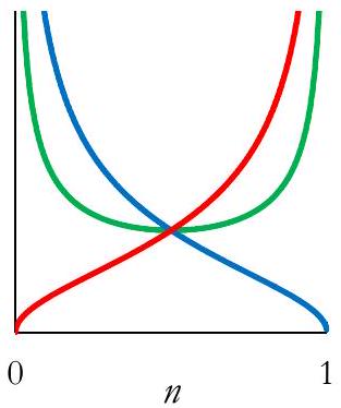
$D^{''} \geq 0$ - the derivative of the damage function is monotonically increasing. In this case, the model is applicable for describing two-stage dependencies with accelerated damage accumulation (Fig. 2, red line).
$D^{''} \leq 0$ - the derivative of the damage function is monotonically decreasing. In this case, the model is applicable for describing two-stage dependencies with decelerated damage accumulation (Fig. 2, blue line).
$D^{''} (n = 0) < 0, D^{''} (n = 1) > 0$ - the derivative of the damage function decreases, reaches a minimum, and then begins to increase. In this case, the model is applicable for describing the well-known three-stage "fast-slow-fast" dependencies (Fig. 2, green line).
$D^{''} (n = 0) > 0, D^{''} (n = 1) < 0$ - the derivative of the damage function increases, reaches a maximum, and then begins to decrease. In this case, the damage function is also three-stage, but corresponds to the "slow-fast-slow" type of dependence, which is not encountered in the literature (Fig. 2, black line). This case will not be considered further.

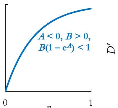
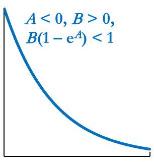
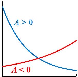
Figure 2: Damage functions

D

, their first derivatives

D^{'}

and second derivatives

D^{''}

: red line

- D^{''} \geq 0

; blue line

- D^{''} \leq 0

; green line

- D^{''} (n = 0) < 0, D^{''} (n = 1) > 0

; black line

- D^{''} (n = 0) > 0, D^{''} (n = 1) < 0

Taking the above into account, the following scheme has been applied for the analysis of phenomenological models of the residual mechanical properties of composites under fatigue damage accumulation:

Identification of the type of function $g_{(β)}$ - linear, power, logarithmic, etc. Based on the type of function, a classification of models can be introduced, since identical functions generally require the same constraints. If the form of the functions $g_{(β)}$ is the same for different models, they are considered equivalent.
Determination of the possibility of representing the damage function in the form of (2) or (3), since in some cases it is impossible to transition from the absolute number of cycles to the relative number (and vice versa) without introducing fatigue life as an additional model parameter.
Verification of the range of the function $g_{(β)} (n)$ within its domain.
Identification of the need to use "normalized damage" (Eq. 4) in the case where $g_{(β)} (n = 1) = 1$ regardless of the values of the model parameters.
Analysis of the positivity of the first derivative of the damage function.
Analysis of the second derivative of the damage function at various parameter values to determine the model's descriptive ability for different stages of damage accumulation.
Determination of the mechanical characteristic $p_{(β)}$ used, the method of calculating its initial value $p_{0} (β)$ , and the dependencies of the model parameters on the cyclic loading parameters - for distinguishing equivalent models. A detailed analysis of the models based on the developed scheme is presented below.

Model analysis. Results

This section analyzes the phenomenological models of residual strength and residual stiffness presented in the literature. Their classification is carried out according to the type of approximating functions used: polynomial, power, logarithmic, exponential, trigonometric, and a group of models based on the use of cumulative distribution functions is also presented.

Polynomial models of residual mechanical characteristics

The general form of models using a polynomial function to predict residual mechanical properties of composites can be represented as follows:

\begin{matrix} (6) & D = A_{0} + A_{1} n + A_{2} n^{2} + \dots + A_{q} n^{q}, q \in N, \end{matrix}

where

A_{i}

are the polynomial coefficients,

q

is the polynomial order. From the condition

D (n = 0) = 0

, it follows that

A_{0} = 0

. Polynomial models are best represented using a relative number of cycles to avoid the occurrence of constants with very small values. The difficulty with using such models is their non-monotonicity, which is why only two polynomial models have found application: linear and quadratic.
Linear and quadratic models. When using a quadratic polynomial, the damage function and its derivatives take the form:

\begin{matrix} (7) & D = A n^{2} + B n, D^{'} = 2 A n + B, D^{''} = 2 A . \end{matrix}

This model does not require the use of "normalized damage", but it is advisable to use a relative number of cycles. The constraints on the function's range and the positivity of the derivative include

0 < B < 2

, while

- 0.5 B < A \leq 1 - B

. Depending on the sign of the parameter

A

, the second derivative takes a positive or negative value throughout the entire domain. Therefore, this model is applicable to describing two-stage dependencies of both types (Fig. 3). It should be noted that higher-order polynomials can be used; however, this would require a significantly larger number of constraints on the parameter values. When

A = 0

, this model is reduced to a linear one, and the damage function and its derivatives take the form:

\begin{matrix} (8) & D = B n, D^{'} = B, D^{''} = 0 \end{matrix}

It should be noted that, unlike the general case of a polynomial model, a linear model can also be used with an absolute value for the number of cycles. Furthermore, this model does not require the use of "normalized damage". The conditions

0 \leq D \leq 1

and

D^{'} > 0

imply the requirement

0 < B \leq 1

.
Obviously, a linear model cannot account for the stage-by-stage nature of damage accumulation processes; however, it is suitable for approximating experimental data corresponding to the stage of gradual damage accumulation. The advantage of this class of models is their ease of use, in particular, the ease of determining the value of parameter

B

. Various versions of quadratic and linear models for the degradation of mechanical properties are known in the literature (Tab. 1, 2).

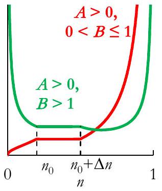
Figure 3: The typical dependencies

D (n)

and

D^{'} (n)

of linear and quadratic models of degradation of residual mechanical characteristics

No	Authors	Year	Model	Additional remarks
Residual stiffness models
1	Andersen S. I. Brondsted P. Lilholt H.	1996 described in [30]	$\frac{S_{R}}{S_{1}} = 1 - A {(\frac{σ_{a}}{E_{0}})}^{B} N, D_{S} = 1 - \frac{S_{R}}{S_{1}} = A {(\frac{σ_{a}}{E_{0}})}^{B} N$	$S_{1}$ is the dynamic Young's modulus at the first cycle; $A, B$ are the experimental fitting parameters
2	Tserpes K. I. Papanikos P. Labeas G. Pantelakis Sp.	2004 [27]	$\frac{S_{R}}{E_{0}} = A n + 1, D_{S} = 1 - \frac{S_{R}}{E_{0}} = - A n$	$A$ is an experimental fitting parameter; CFRP with the thermosetting resin ${[45^{\circ} / 0^{\circ} / - 45^{\circ} / 90^{\circ}]}_{25}$ and the thermoplastic resin $[45^{\circ} / 0^{\circ} / - {45^{\circ} / 90^{\circ}_{2} / - 45^{\circ} / 0^{\circ} / 45^{\circ}]}_{s}$ , cyclic tension-compression, $R = - 1$
Residual strength models
3	Broutman L. J. Sahu S.	1972 [36]	$σ_{R} = σ_{U} - (σ_{U} - σ_{max}) n, D_{σ}^{*} = \frac{σ_{U} - σ_{R}}{σ_{U} - σ_{max}} = n$	GFRP, cyclic tension, $R = 0.05$ , 150-1500 cycle/min
$\frac{σ_{R}}{σ_{U}} = 1 - A {(\frac{σ_{max}}{σ_{U}})}^{B} N$ ,
4	Strizhius V.	2022 [37]	$D_{σ} = 1 - \frac{σ_{R}}{σ_{U}} = A {(\frac{σ_{max}}{σ_{U}})}^{B} N, A = \frac{1 - \frac{σ_{max}}{σ_{U}}}{{(\frac{σ_{max}}{σ_{U}})}^{B} N_{f}}$	CFRP ${[0^{\circ} / \pm 45^{\circ} / 90^{\circ}]}_{s 4}$ with open hole, cyclic tension and compression

Table 1: Linear models of degradation of residual mechanical properties.

No	Authors	Year	Model	Additional remarks
Residual strength models
1	Owen M. J., Howe R. J.	1972 [38]	$\frac{σ_{R}}{σ_{U}} = 1 - B n + A n^{2}, D_{σ} = 1 - \frac{σ_{R}}{σ_{U}} = B n - A n^{2}$	GFRP, cyclic tension, 100 cycle/min
2	Tserpes K. I. Papanikos P. Labeas G. Pantelakis Sp.	2004 [27]	$\frac{σ_{R}}{σ_{U}} = A n^{2} + B n + 1, D_{σ} = 1 - \frac{σ_{R}}{σ_{U}} = - A n^{2} - B n$	$A, B$ are the experimental fitting parameters; CFRP with the thermosetting resin ${[45^{\circ} / 0^{\circ} / - 45^{\circ} / 90^{\circ}]}_{25}$ and the thermoplastic resin $[45^{\circ} / 0^{\circ} / - 45^{\circ} / 90^{\circ}_{2} / - 45^{\circ} / 0^{\circ} / 45^{\circ}] s$ , cyclic tension-compression, $R = - 1$

Table 2: Quadratic models of degradation of residual mechanical properties.

Power law models of residual mechanical characteristics

Power functions and their combinations have been successfully used by researchers for many years to approximate experimental data on the degradation of residual mechanical properties. Therefore, this group is the most numerous one. Simple power law models. A simple power law model can be represented as:

\begin{matrix} (9) & D = A n^{B}, D^{'} = A B n^{B - 1}, D^{''} = A B (B - 1) n^{B - 2} . \end{matrix}

In this case, either the absolute or relative number of cycles can be used, and there is no requirement for the use of "normalized damage". Using the simple power law model requires the following constraints on the parameter values:

0 < A < 1, B > 0, B \neq 1

(otherwise, the model is reduced to a linear model). Depending on the value of parameter

B

, two options can be implemented (Fig. 4):

when $0 < B < 1$ , then $D^{''} < 0$ , which corresponds to a two-stage dependence with decelerated damage accumulation;
when $B > 1$ , then $D^{''} > 0$ , which corresponds to a two-stage dependence with accelerated damage accumulation.

Figure 4: The typical dependencies

D (n)

and

D^{'} (n)

of power law models of degradation of residual mechanical characteristics.

The advantage of simple power law models is their ease of use, particularly the ease of determining the values of parameters

A

and

B

, as well as their greater descriptive ability compared to linear models. A disadvantage of these models is their inability to describe three-stage dependencies. Various applications of the simple power law model for the degradation of residual mechanical properties are known in the literature, as summarized in Tab. 3.

Figure 4: The typical dependencies

D (n)

and

D^{'} (n)

of power law models of degradation of residual mechanical characteristics.

Authors

Year

Model

Additional remarks

Residual stiffness models

Wang S. S., Chim E. S. M.

1983 [31]

D_{S} = 1 - \frac{S_{R}}{S_{10}} = A N^{B}, B = b_{0} + b_{1} σ_{max} + b_{2} σ_{max}^{2} + \dots

short-fiber glass composite, cyclic tension

Hwang W., Han K. S.

1986 [16]

D_{F}^{*} = \frac{F_{0} - F_{R}}{F_{0} - F_{f}} = n^{B}

F_{0}

is the initial fatigue modulus that assumed to be the same as elastic modulus

E_{0} (F_{0} \approx E_{0})

Yang J. N., Jones D. L., Yang S. H., Meskini A.

1990 [39]

\begin{matrix} \frac{S_{R}}{S_{0}} = 1 - A N^{B}, D_{S} = 1 - \frac{S_{R}}{S_{0}} = A N^{B} \\ A = A_{1} + A_{2} B, B = A_{3} + C σ_{max} \end{matrix}

S_{0}

is the initial stiffness measured at a loading rate of 4 Hz ;

A, B

are the random variables that depend on the applied stress level;

C

is a random variable;

A_{1}, A_{2}, A_{3}

are the parameters independent of applied stress level; fiber dominated composite (graphite/epoxy laminates) [

90 / + 45 / - 45 / 0]_{s}

, cyclic tension,

10 Hz, R = 0.1

Yang J. N., Lee L. J., Sheu D. Y.

1992 [40]

\begin{aligned} \frac{F_{R}}{F_{1}} & = 1 - A N^{B}, D_{F} = 1 - \frac{F_{R}}{F_{1}} = A N^{B} \\ A & = A_{1} + A_{2} B, B = A_{3} + C σ_{max} \end{aligned}

F_{1}

is the initial fatigue modulus at the first cycle; matrix dominated composite (graphite/epoxy laminates

[\pm 45]_{2 s}

), cyclic tension,

10 Hz, R = 0.1

Authors

Year

Model

Additional remarks

Passipoularidis V. A. Philippidis T. P. Brondsted P.

2011 described in [41]

\frac{S_{R}}{E_{0}} = 1 - (1 - A) n^{B}, D_{S} = 1 - \frac{S_{R}}{E_{0}} = (1 - A) n^{B}

A, B

are the constant parameters fitted to stiffness measurements taken during fatigue testing

Laribi M.A. Tamboura S. Fitoussi J. Tié Bi R. Tcharkhtchi A. Ben Dali H.

2018 [42]

\begin{matrix} \frac{S_{R}}{E_{0}} = [1 + A (σ_{max} - σ_{S})] {(\frac{N}{N_{S}})}^{B}, \\ D_{S} = 1 - \frac{S_{R}}{E_{0}} = 1 - [1 + A (σ_{max} - σ_{S})] {(\frac{N}{N_{S}})}^{B} \end{matrix}

σ_{S}

is the average damage threshold stress until which there is no relative loss of stiffness;

N_{S}

is the number of cycles until which there is no evolution of the relative loss of stiffness;

sheet molding compound composite, cyclic tension,

R = 0.1, 10 Hz

Residual strength models

Stinchcomb W. W., Reifsnider K. L.

1986 described in [43]

\begin{aligned} σ_{R} & = σ_{U} - (σ_{U} - σ_{max}) n^{A}, \\ D_{σ} & = 1 - \frac{σ_{R}}{σ_{U}} = (1 - \frac{σ_{max}}{σ_{U}}) n^{A}, \end{aligned}

Shaff J. R., Davidson B. D.

1997 [44, 45]

A = 1

linear strength degradation;

A ≫ 1

"sudden death" behavior;

A < 1

rapid initial loss in strength; cross-ply glass/epoxy laminates, cyclic tension

D'Amore A., Carpino G., Stupak P., Zhou J., Nicolais L.

1996 [46]

\begin{matrix} σ_{R} = σ_{U} - \frac{A}{1 - B} σ_{max} (1 - R) (N^{1 - B} - 1), \\ D_{σ} = 1 - \frac{σ_{R}}{σ_{U}} = \frac{A}{(1 - B)} \frac{σ_{max}}{σ_{U}} (1 - R) (N^{1 - B} - 1) \end{matrix}

A, B

are the constants dependent on the material type and load conditions;

R

is a stress ratio; GFRP, polyester/ polyurethane resin, four-point bending fatigue,

0, 8 - 2 Hz

R = 0, 1, 0, 3, 0, 5, 0, 7

D'Amore A., Giorgio M., Grassia L.

2015 [47]

\begin{aligned} σ_{R} = σ_{max} + \frac{A}{1 - B} σ_{max} (1 - R) (N_{f}^{1 - B} - N^{1 - B}), \\ D_{σ} = 1 - \frac{σ_{R}}{σ_{U}} = \frac{A}{(1 - B)} \frac{σ_{max}}{σ_{U}} (1 - R) (N^{1 - B} - 1) \end{aligned},

Ganesan C., Joanna P.S.

2018 [48]

\begin{matrix} σ_{R} = σ_{U} + \frac{A}{1 - B} σ_{max} (1 - R) (1 - (1 + N)^{1 - B}), \\ D_{σ} = 1 - \frac{σ_{R}}{σ_{U}} = - \frac{A}{1 - B} \frac{σ_{max}}{σ_{U}} (1 - R) (1 - (1 + N)^{1 - B}) \end{matrix}

woven GFRP, cyclic tension,

R = 0.5, 3 Hz

Epaarachchi J.A., Clausen P.D.

2003, 2005 [49, 50]

\begin{aligned} σ_{U} - σ_{R} & = \frac{A}{f^{C}} {(\frac{σ_{max}}{σ_{U}})}^{0.6 - B | \sin θ |} [σ_{max} (1 - B)^{1.6 - B | \sin θ |}] (N^{C} - 1), \\ D_{σ} & = 1 - \frac{σ_{R}}{σ_{U}} = \frac{A}{f^{C}} {[\frac{σ_{max}}{σ_{U}} (1 - B)]}^{1.6 - B | \sin θ |} (N^{C} - 1) \end{aligned}

f

is the frequency;

θ

is the smallest ply angle of the laminate to the loading direction;

A, B

are the material parameters;

B = R

(stress ratio) for

- \infty \leq R \leq 1

B = 1 / R

for

1 < R \leq \infty

No Authors Year Model Additional remarks 5 Passipoularidis V. A. Philippidis T. P. Brondsted P. 2011 described in [41] (S_(R))/(E_(0))=1-(1-A)n^(B),quadD_(S)=1-(S_(R))/(E_(0))=(1-A)n^(B) A,B are the constant parameters fitted to stiffness measurements taken during fatigue testing 6 Laribi M.A. Tamboura S. Fitoussi J. Tié Bi R. Tcharkhtchi A. Ben Dali H. 2018 [42] "(S_(R))/(E_(0))=[1+A(sigma_(max)-sigma_(S))]((N)/(N_(S)))^(B), D_(S)=1-(S_(R))/(E_(0))=1-[1+A(sigma_(max)-sigma_(S))]((N)/(N_(S)))^(B)" "sigma_(S) is the average damage threshold stress until which there is no relative loss of stiffness; N_(S) is the number of cycles until which there is no evolution of the relative loss of stiffness; sheet molding compound composite, cyclic tension, R=0.1,10Hz" Residual strength models 7 Stinchcomb W. W., Reifsnider K. L. 1986 described in [43] "sigma_(R)=sigma_(U)-(sigma_(U)-sigma_(max))n^(A), D_(sigma)=1-(sigma_(R))/(sigma_(U))=(1-(sigma_(max))/(sigma_(U)))n^(A)," - 8 Shaff J. R., Davidson B. D. 1997 [44, 45] A=1 linear strength degradation; A≫1 "sudden death" behavior; A < 1 rapid initial loss in strength; cross-ply glass/epoxy laminates, cyclic tension 9 D'Amore A., Carpino G., Stupak P., Zhou J., Nicolais L. 1996 [46] "sigma_(R)=sigma_(U)-(A)/(1-B)sigma_(max)(1-R)(N^(1-B)-1), D_(sigma)=1-(sigma_(R))/(sigma_(U))=(A)/((1-B))(sigma_(max))/(sigma_(U))(1-R)(N^(1-B)-1)" A,B are the constants dependent on the material type and load conditions; R is a stress ratio; GFRP, polyester/ polyurethane resin, four-point bending fatigue, 0,8-2Hz, R=0,1,0,3,0,5,0,7 10 D'Amore A., Giorgio M., Grassia L. 2015 [47] "sigma_(R)=sigma_(max)+(A)/(1-B)sigma_(max)(1-R)(N_(f)^(1-B)-N^(1-B)), D_(sigma)=1-(sigma_(R))/(sigma_(U))=(A)/((1-B))(sigma_(max))/(sigma_(U))(1-R)(N^(1-B)-1)", - 11 Ganesan C., Joanna P.S. 2018 [48] "sigma_(R)=sigma_(U)+(A)/(1-B)sigma_(max)(1-R)(1-(1+N)^(1-B)), D_(sigma)=1-(sigma_(R))/(sigma_(U))=-(A)/(1-B)(sigma_(max))/(sigma_(U))(1-R)(1-(1+N)^(1-B))" woven GFRP, cyclic tension, R=0.5,3Hz 12 Epaarachchi J.A., Clausen P.D. 2003, 2005 [49, 50] "sigma_(U)-sigma_(R)=(A)/(f^(C))((sigma_(max))/(sigma_(U)))^(0.6-B|sin theta|)[sigma_(max)(1-B)^(1.6-B|sin theta|)](N^(C)-1), D_(sigma)=1-(sigma_(R))/(sigma_(U))=(A)/(f^(C))[(sigma_(max))/(sigma_(U))(1-B)]^(1.6-B|sin theta|)(N^(C)-1)" f is the frequency; theta is the smallest ply angle of the laminate to the loading direction; A,B are the material parameters; B=R (stress ratio) for -oo <= R <= 1, B=1//R for 1 < R <= oo

| No | Authors | Year | Model | Additional remarks | | :--- | :--- | :--- | :--- | :--- | | 5 | Passipoularidis V. A. Philippidis T. P. Brondsted P. | 2011 described in [41] | $\frac{S_{R}}{E_{0}}=1-(1-A) n^{B}, \quad D_{S}=1-\frac{S_{R}}{E_{0}}=(1-A) n^{B}$ | $A, B$ are the constant parameters fitted to stiffness measurements taken during fatigue testing | | 6 | Laribi M.A. Tamboura S. Fitoussi J. Tié Bi R. Tcharkhtchi A. Ben Dali H. | 2018 [42] | $\begin{gathered} \frac{S_{\mathrm{R}}}{E_{0}}=\left[1+A\left(\sigma_{\max }-\sigma_{S}\right)\right]\left(\frac{N}{N_{S}}\right)^{B}, \\ D_{S}=1-\frac{S_{\mathrm{R}}}{E_{0}}=1-\left[1+A\left(\sigma_{\max }-\sigma_{S}\right)\right]\left(\frac{N}{N_{S}}\right)^{B} \end{gathered}$ | $\sigma_{S}$ is the average damage threshold stress until which there is no relative loss of stiffness; $N_{S}$ is the number of cycles until which there is no evolution of the relative loss of stiffness; sheet molding compound composite, cyclic tension, $R=0.1,10 \mathrm{~Hz}$ | | Residual strength models | | | | | | 7 | Stinchcomb W. W., Reifsnider K. L. | 1986 described in [43] | $\begin{aligned} \sigma_{R} & =\sigma_{U}-\left(\sigma_{U}-\sigma_{\max }\right) n^{A}, \\ D_{\sigma} & =1-\frac{\sigma_{R}}{\sigma_{U}}=\left(1-\frac{\sigma_{\max }}{\sigma_{U}}\right) n^{A}, \end{aligned}$ | - | | 8 | Shaff J. R., Davidson B. D. | 1997 [44, 45] | | $A=1$ linear strength degradation; $A \gg 1$ "sudden death" behavior; $A<1$ rapid initial loss in strength; cross-ply glass/epoxy laminates, cyclic tension | | 9 | D'Amore A., Carpino G., Stupak P., Zhou J., Nicolais L. | 1996 [46] | $\begin{gathered} \sigma_{R}=\sigma_{U}-\frac{A}{1-B} \sigma_{\max }(1-R)\left(N^{1-B}-1\right), \\ D_{\sigma}=1-\frac{\sigma_{R}}{\sigma_{U}}=\frac{A}{(1-B)} \frac{\sigma_{\max }}{\sigma_{U}}(1-R)\left(N^{1-B}-1\right) \end{gathered}$ | $A, B$ are the constants dependent on the material type and load conditions; $R$ is a stress ratio; GFRP, polyester/ polyurethane resin, four-point bending fatigue, $0,8-2 \mathrm{~Hz}$, $R=0,1,0,3,0,5,0,7$ | | 10 | D'Amore A., Giorgio M., Grassia L. | 2015 [47] | $\begin{aligned} & \sigma_{\mathrm{R}}=\sigma_{\max }+\frac{A}{1-B} \sigma_{\max }(1-\mathrm{R})\left(N_{f}^{1-B}-N^{1-B}\right), \\ & D_{\sigma}=1-\frac{\sigma_{\mathrm{R}}}{\sigma_{U}}=\frac{A}{(1-B)} \frac{\sigma_{\max }}{\sigma_{U}}(1-\mathrm{R})\left(N^{1-B}-1\right) \end{aligned},$ | - | | 11 | Ganesan C., Joanna P.S. | 2018 [48] | $\begin{gathered} \sigma_{\mathrm{R}}=\sigma_{U}+\frac{A}{1-B} \sigma_{\max }(1-\mathrm{R})\left(1-(1+N)^{1-B}\right), \\ D_{\sigma}=1-\frac{\sigma_{\mathrm{R}}}{\sigma_{U}}=-\frac{A}{1-B} \frac{\sigma_{\max }}{\sigma_{U}}(1-\mathrm{R})\left(1-(1+N)^{1-B}\right) \end{gathered}$ | woven GFRP, cyclic tension, $R=0.5,3 \mathrm{~Hz}$ | | 12 | Epaarachchi J.A., Clausen P.D. | 2003, 2005 [49, 50] | $\begin{aligned} \sigma_{U}-\sigma_{\mathrm{R}} & =\frac{A}{f^{C}}\left(\frac{\sigma_{\max }}{\sigma_{U}}\right)^{0.6-B\|\sin \theta\|}\left[\sigma_{\max }(1-B)^{1.6-B\|\sin \theta\|}\right]\left(N^{C}-1\right), \\ D_{\sigma} & =1-\frac{\sigma_{\mathrm{R}}}{\sigma_{U}}=\frac{A}{f^{C}}\left[\frac{\sigma_{\max }}{\sigma_{U}}(1-B)\right]^{1.6-B\|\sin \theta\|}\left(N^{C}-1\right) \end{aligned}$ | $f$ is the frequency; $\theta$ is the smallest ply angle of the laminate to the loading direction; $A, B$ are the material parameters; $B=R$ (stress ratio) for $-\infty \leq R \leq 1$, $B=1 / R$ for $1<R \leq \infty$ |

Table 3: Power law models of degradation of residual mechanical properties

Power law models of Hahn H. T. and Kim R. Y. type. Hahn H. T. and Kim R. Y. [51] proposed using the following expression to determine the residual strength:

\begin{matrix} (10) & σ_{R}^{A} = σ_{U}^{A} - A B N, \end{matrix}

where

A

is the constant,

B

is the parameter, which depends on the characteristics of fatigue loading (considering a single stress level,

B

is treated as a constant). This expression can be considered an analogue of the linear model if the residual mechanical characteristic is considered to be

σ_{R}^{A}

. However, it can be shown that this model can be reduced to the following form:

\begin{matrix} (11) & D_{σ} = 1 - \frac{σ_{R}}{σ_{U}} = 1 - (1 - A n)^{B}, D^{'} = A B (1 - A n)^{B - 1}, D^{''} = - A^{2} B (B - 1) (1 - A n)^{B - 2}, \end{matrix}

where

A, B

are the model parameters dependent on loading conditions. The model can be represented as a function of both the absolute and relative number of cycles, and it is possible to take into account the residual value of the mechanical characteristic before fatigue failure. The constraints on the range of the function imply that

A < 1

, with

A \neq 0

. When

B = 1

, this model is linear. The constraints on the positivity of the first derivative of the damage function imply that

A B > 0

. Various options for using this power law model for the degradation of residual mechanical properties are presented in Tab. 4. Depending on the value of parameter

B

, the following situations are possible (Fig. 5):

when $0 0$ , which corresponds to a two-stage dependence with accelerated damage accumulation;
when $B < 0$ or $B > 1$ , then $D^{''} < 0$ , which corresponds to a two-stage dependence with decelerated damage accumulation.

Authors

Year

Model

Additional remarks

Residual strength models

Hahn H. T., Kim R. Y.

1975 [51]

σ_{R}^{A} = σ_{U}^{A} - A B N, D_{σ} = 1 - \frac{σ_{R}}{σ_{U}} = 1 - {(1 - \frac{A B}{σ_{U}^{A}} N)}^{\frac{1}{A}}

A

is a constant;

B

is a parameter, which depends on the characteristics of fatigue loading

Yang J. N., Liu M. D.

1977 [52]

\begin{matrix} σ_{R}^{C} = σ_{U}^{C} - A β^{C} σ_{max}^{B} N, \\ D_{σ} = 1 - \frac{σ_{R}}{σ_{U}} = 1 - {(1 - \frac{A β^{C} σ_{max}^{B}}{σ_{U}^{C}} N)}^{\frac{1}{C}} \end{matrix}

A, B, C

are the experimental fitting parameters;

B

is a parameter of the statistical distribution of initial strength data; graphite/epoxy laminate

[0 / 90 / \pm 45]_{s}, 20 Hz, R = 0.1

Yang J. N., Sun C. T.

1980

[53]

\begin{matrix} σ_{R}^{V} = σ_{U}^{V} - \frac{σ_{U}^{V} - σ_{max}^{V}}{σ_{U}^{C} - σ_{max}^{C}} A σ_{range}^{B} N, \\ D_{σ} = 1 - \frac{σ_{R}}{σ_{U}} = 1 - {(1 - A \frac{σ_{range}^{B}}{σ_{U}^{V}} \frac{σ_{U}^{V} - σ_{max}^{V}}{σ_{U}^{C} - σ_{max}^{C}} N)}^{\frac{1}{V}} \end{matrix}

σ_{R}, σ_{U}, σ_{max}

are the characteristics normalized by

β

;

V

is a parameter determining the rate of strength degradation;

A, B

are the parameters of the

S - N

curve for the characteristic fatigue life

σ_{R}^{A} = σ_{U}^{A} - (σ_{U}^{A} - σ_{max}^{A}) n

Hashin Z.

1985

[54]

D_{σ} = 1 - \frac{σ_{R}}{σ_{U}} = 1 - {[1 - (1 - \frac{σ_{max}^{A}}{σ_{U}^{A}}) n]}^{\frac{1}{A}}

A

is an empirical parameter

σ_{R}^{A} = σ_{U}^{A} - B σ_{max}^{A} (N - 1)

Sendeckyj

G. P.

1991

[55]

\begin{matrix} σ_{R}^{A} = σ_{U}^{A} - B σ_{max}^{A} (N - 1), \\ D_{σ} = 1 - \frac{σ_{R}}{σ_{U}} = 1 - {[1 - B (N - 1) {(\frac{σ_{max}}{σ_{U}})}^{A}]}^{\frac{1}{A}} \end{matrix}

A, B

are the two dimensionless functions that do not depend on

σ

Whitworth

2000 H. A.

[56]

σ_{R}^{C} = σ_{U}^{C} - (σ_{U}^{C} - σ_{max}^{C}) \frac{N}{N_{f}},

D_{σ} = 1 - \frac{σ_{R}}{σ_{U}} = 1 - {[1 - \frac{(1 - \frac{σ_{max}^{C}}{σ_{U}^{C}}) N}{\exp {\frac{1}{A} [{(\frac{B σ_{U}}{σ_{max}})}^{V / C} - 1]} - 1}]}^{\frac{1}{C}}

A, V

are the parameters that depends on the applied stress;

B, C

are the experimentally determined constants

No Authors Year Model Additional remarks Residual strength models 1 Hahn H. T., Kim R. Y. 1975 [51] sigma_(R)^(A)=sigma_(U)^(A)-ABN,quadD_(sigma)=1-(sigma_(R))/(sigma_(U))=1-(1-(AB)/(sigma_(U)^(A))N)^((1)/(A)) A is a constant; B is a parameter, which depends on the characteristics of fatigue loading 2 Yang J. N., Liu M. D. 1977 [52] "sigma_(R)^(C)=sigma_(U)^(C)-Abeta^(C)sigma_(max)^(B)N, D_(sigma)=1-(sigma_(R))/(sigma_(U))=1-(1-(Abeta^(C)sigma_(max)^(B))/(sigma_(U)^(C))N)^((1)/(C))" "A,B,C are the experimental fitting parameters; B is a parameter of the statistical distribution of initial strength data; graphite/epoxy laminate [0//90//+-45]_(s),20Hz,R=0.1" 3 Yang J. N., Sun C. T. "1980 [53]" "sigma_(R)^(V)=sigma_(U)^(V)-(sigma_(U)^(V)-sigma_(max)^(V))/(sigma_(U)^(C)-sigma_(max)^(C))Asigma_(range )^(B)N, D_(sigma)=1-(sigma_(R))/(sigma_(U))=1-(1-A(sigma_(range )^(B))/(sigma_(U)^(V))(sigma_(U)^(V)-sigma_(max)^(V))/(sigma_(U)^(C)-sigma_(max)^(C))N)^((1)/(V))" "sigma_(R),sigma_(U),sigma_("max ") are the characteristics normalized by beta; V is a parameter determining the rate of strength degradation; A,B are the parameters of the S-N curve for the characteristic fatigue life" 4 sigma_(R)^(A)=sigma_(U)^(A)-(sigma_(U)^(A)-sigma_("max ")^(A))n, Hashin Z. "1985 [54]" D_(sigma)=1-(sigma_(R))/(sigma_(U))=1-[1-(1-(sigma_("max ")^(A))/(sigma_(U)^(A)))n]^((1)/(A)) A is an empirical parameter 5 sigma_(R)^(A)=sigma_(U)^(A)-Bsigma_("max ")^(A)(N-1), "Sendeckyj G. P." "1991 [55]" "sigma_(R)^(A)=sigma_(U)^(A)-Bsigma_(max)^(A)(N-1), D_(sigma)=1-(sigma_(R))/(sigma_(U))=1-[1-B(N-1)((sigma_(max))/(sigma_(U)))^(A)]^((1)/(A))" A,B are the two dimensionless functions that do not depend on sigma 6 "Whitworth 2000 H. A. [56]" sigma_(R)^(C)=sigma_(U)^(C)-(sigma_(U)^(C)-sigma_(max)^(C))(N)/(N_(f)), D_(sigma)=1-(sigma_(R))/(sigma_(U))=1-[1-((1-(sigma_("max ")^(C))/(sigma_(U)^(C)))N)/(exp{(1)/(A)[((Bsigma_(U))/(sigma_("max ")))^(V//C)-1]}-1)]^((1)/(C)) A,V are the parameters that depends on the applied stress; B,C are the experimentally determined constants

| No | Authors | Year | Model | Additional remarks | | :--- | :--- | :--- | :--- | :--- | | Residual strength models | | | | | | 1 | Hahn H. T., Kim R. Y. | 1975 [51] | $\sigma_{R}^{A}=\sigma_{U}^{A}-A B N, \quad D_{\sigma}=1-\frac{\sigma_{R}}{\sigma_{U}}=1-\left(1-\frac{A B}{\sigma_{U}^{A}} N\right)^{\frac{1}{A}}$ | $A$ is a constant; $B$ is a parameter, which depends on the characteristics of fatigue loading | | 2 | Yang J. N., Liu M. D. | | | | | | | 1977 [52] | $\begin{gathered} \sigma_{R}^{C}=\sigma_{U}^{C}-A \beta^{C} \sigma_{\max }^{B} N, \\ D_{\sigma}=1-\frac{\sigma_{R}}{\sigma_{U}}=1-\left(1-\frac{A \beta^{C} \sigma_{\max }^{B}}{\sigma_{U}^{C}} N\right)^{\frac{1}{C}} \end{gathered}$ | $A, B, C$ are the experimental fitting parameters; $B$ is a parameter of the statistical distribution of initial strength data; graphite/epoxy laminate $[0 / 90 / \pm 45]_{\mathrm{s}}, 20 \mathrm{~Hz}, \mathrm{R}=0.1$ | | 3 | Yang J. N., Sun C. T. | 1980 [53] | $\begin{gathered} \sigma_{R}^{V}=\sigma_{U}^{V}-\frac{\sigma_{U}^{V}-\sigma_{\max }^{V}}{\sigma_{U}^{C}-\sigma_{\max }^{C}} A \sigma_{\text {range }}^{B} N, \\ D_{\sigma}=1-\frac{\sigma_{R}}{\sigma_{U}}=1-\left(1-A \frac{\sigma_{\text {range }}^{B}}{\sigma_{U}^{V}} \frac{\sigma_{U}^{V}-\sigma_{\max }^{V}}{\sigma_{U}^{C}-\sigma_{\max }^{C}} N\right)^{\frac{1}{V}} \end{gathered}$ | $\sigma_{\mathrm{R}}, \sigma_{\mathrm{U}}, \sigma_{\text {max }}$ are the characteristics normalized by $\beta$; $V$ is a parameter determining the rate of strength degradation; $A, B$ are the parameters of the $S-N$ curve for the characteristic fatigue life | | 4 | | | $\sigma_{R}^{A}=\sigma_{U}^{A}-\left(\sigma_{U}^{A}-\sigma_{\text {max }}^{A}\right) n$, | | | | Hashin Z. | 1985 [54] | $D_{\sigma}=1-\frac{\sigma_{R}}{\sigma_{U}}=1-\left[1-\left(1-\frac{\sigma_{\text {max }}^{A}}{\sigma_{U}^{A}}\right) n\right]^{\frac{1}{A}}$ | $A$ is an empirical parameter | | 5 | | | $\sigma_{R}{ }^{A}=\sigma_{U}{ }^{A}-B \sigma_{\text {max }}{ }^{A}(N-1)$, | | | | Sendeckyj G. P. | 1991 [55] | $\begin{gathered} \sigma_{R}^{A}=\sigma_{U}^{A}-B \sigma_{\max }^{A}(N-1), \\ D_{\sigma}=1-\frac{\sigma_{R}}{\sigma_{U}}=1-\left[1-B(N-1)\left(\frac{\sigma_{\max }}{\sigma_{U}}\right)^{A}\right]^{\frac{1}{A}} \end{gathered}$ | $A, B$ are the two dimensionless functions that do not depend on $\sigma$ | | 6 | Whitworth 2000 H. A. [56] | | $\sigma_{R}^{C}=\sigma_{U}^{C}-\left(\sigma_{U}^{C}-\sigma_{\max }^{C}\right) \frac{N}{N_{f}},$ $D_{\sigma}=1-\frac{\sigma_{R}}{\sigma_{U}}=1-\left[1-\frac{\left(1-\frac{\sigma_{\text {max }}^{C}}{\sigma_{U}^{C}}\right) N}{\exp \left\{\frac{1}{A}\left[\left(\frac{B \sigma_{U}}{\sigma_{\text {max }}}\right)^{V / C}-1\right]\right\}-1}\right]^{\frac{1}{C}}$ | | | | | | $A, V$ are the parameters that depends on the applied stress; $B, C$ are the experimentally determined constants | | | | | |

Table 4: Power law models of the type of Hahn H. T., Kim R. Y.

Figure 5: The typical dependencies

D (n)

and

D^{'} (n)

of Hahn H. T., Kim R. Y. type power law model.

Tang H. C., Nguyen T., Chuang T., Chin J., Lesko J. and Wu H. F. model. The authors [57] proposed a general model of stiffness degradation, approximating the initial and final sections of the damage dependence on the number of cycles in the form:

\begin{matrix} (12) & D_{E} = 1 - \frac{E_{R}}{E_{0}}, \frac{d D_{E}}{d N} = \frac{A_{1}}{D_{E}^{B_{1}}} + \frac{A_{2}}{{(1 - D_{E})}^{B_{2}}} . \end{matrix}

Here,

A_{1}, A_{2}, B_{1}, B_{2}

are model parameters selected experimentally. The authors propose using the first term of the sum to describe the initial section of the stiffness degradation diagram, and the second term for the final section. It is noted that this differential equation cannot be solved explicitly. Therefore, a simplified model consisting of one of the two terms can be considered, assuming

A_{1} = 0

A_{2} = 0

. It can be shown that when

A_{2} = 0

, this model reduces to the simple power law (Eq. 9), and when

A_{1} = 0

, this model reduces to the general form (Eq. 11).
Wu F., Yao W.X. and Stojković N., Folić R, Pasternak H. model. Wu F. and Yao W.X. [28] proposed using the following combination of power functions to approximate the residual Young's modulus data:

\begin{matrix} (13) & D_{E}^{*} = \frac{E_{0} - E_{R}}{E_{0} - E_{f}} = 1 - {(1 - n^{B})}^{A}, A = 1 + (B - 1) \frac{\lg \frac{n_{1}}{n_{2}}}{\lg \frac{1 - n_{2}^{B}}{1 - n_{1}^{B}}}, B = k \frac{\lg N_{f}}{(1 - R) \frac{σ_{max}}{σ_{U}}}, \end{matrix}

where

A, B

are the linearly related model parameters;

n_{1}, n_{2}

are the values of

n

corresponding to the boundaries of the second stage of damage accumulation

(0 < n_{1} < n_{2} < 1); k

is the proportionality coefficient;

R

is the cycle ratio.
For the residual strength, Stojković N., Folić R., Pasternak H. [58] used the model of Shaff J. R., Davidson B. D. [44, 45] and introduced the concept of strength reserve

σ_{res}

\begin{matrix} (14) & σ_{R} = σ_{U} - (σ_{U} - σ_{max}) n^{B}, σ_{r e s} = σ_{R} - σ_{max} = (σ_{U} - σ_{max}) (1 - n^{B}), \end{matrix}

and then, for three-stage dependencies, they proposed using a combination of power functions, called the normalized strength reserve model, which, when transformed, yields the expression:

\begin{matrix} (15) & σ_{r e s, n} = \frac{σ_{R} - σ_{max}}{σ_{U} - σ_{max}} = {(1 - n^{B})}^{A}, σ_{R} = σ_{max} + (σ_{U} - σ_{max}) {(1 - n^{B})}^{A}, D_{σ}^{*} = \frac{σ_{U} - σ_{R}}{σ_{U} - σ_{max}} = 1 - {(1 - n^{B})}^{A} \end{matrix}

Thus, the general form of the model and its derivatives is:

\begin{aligned} D = 1 - {(1 - n^{B})}^{A}, D^{'} = A B {(1 - n^{B})}^{A - 1} n^{B - 1}, \\ (16) & D^{''} = A B [- (A - 1) B {(1 - n^{B})}^{A - 2} n^{2 B - 2} + (B - 1) {(1 - n^{B})}^{A - 1} n^{B - 2}] . \end{aligned}

It should be noted that the model is only applicable when using the relative number of cycles and "normalized damage". The constraints on the range of values of the function imply that

A > 0

and

B > 0

. In this case, for

A = 1

, the model reduces to a simple power function, while for

B = 1

, it is a model of type (Eq. 11).
Since

A, B > 0

, the condition for the first derivative to be positive is satisfied. Depending on the values of parameters

A

and

B

, the following options are possible (Tab. 5):

when $A < 1$ and $B \geq 1$ , then $D^{''} \geq 0$ and the function is applicable to describing two-stage dependencies with accelerated damage accumulation;
when $A > 1$ and $B \leq 1$ , then $D^{''} \leq 0$ and the function is applicable to describing two-stage dependencies with decelerated damage accumulation;
when $A < 1$ and $B < 1$ , then the function is suitable for describing three-stage "fast-slow-fast" dependencies;
when $A > 1$ and $B > 1$ , then the function is suitable for describing three-stage "slow-fast-slow" dependencies. Model of Yang J. N. and Du S. type. The authors [59] proposed the following equation for predicting the residual strength of polymer composites:

\begin{matrix} (17) & σ_{R}^{V} = σ_{U}^{V} - \frac{σ_{U}^{V} - σ_{max}^{V}}{{(σ_{U}^{C} - σ_{max}^{C})}^{Y}} {(A σ_{range}^{B} N)}^{Y}, \end{matrix}

where

σ_{R}

is the residual strength normalized by

β; σ_{max}

is the maximum fatigue stress normalized by

β; V, A, B, C

and

Y

are the model parameters;

σ_{rang}

is the stress range. This expression can be reduced to the following form:

\begin{aligned} (18) & D_{σ} & = 1 - \frac{σ_{R}}{σ_{U}} = 1 - {(1 - A n^{B})}^{C}, D^{'} = A B C {(1 - A n^{B})}^{C - 1} n^{B - 1}, \\ D^{''} & = A B C {(1 - A n^{B})}^{C - 2} n^{B - 2} (A n^{B} (1 - B C) + B - 1) . \end{aligned}

Here,

A, B

, and

C

are model parameters dependent on loading conditions. The model can be represented as a function of either the absolute or the relative number of cycles, and it is possible to take into account the residual value of the mechanical characteristic before fatigue failure. The constraints on the range of the function imply that

A \leq 1

, with

A \neq 0, B > 0, C \neq 0

. The following cases are possible:

when $B = C = 1$ , this model reduces to a linear model (Eq. 8);
when $B \neq 1$ and $C = 1$ , this model reduces to a simple power law model (Eq. 9);
when $B = 1$ and $C \neq 1$ , this model reduces to models of the type of Hahn H. T., Kim R. Y. [51] (Eq. 11);
when $A = 1$ , this model reduces to the model Stojković N., Folić R., Pasternak H. [58] (Eq. 16).

Accordingly, this model (Eq. 18) can be called a generalization of previously presented types of models, as proposed by Sarkani S., Michaelov G., Kihl D. P., Bonanni D. L [10].
From the constraints on the positivity of the first derivative of the damage function it follows that

A C > 0

. Depending on the values of the model parameters, the following cases are possible (Tab. 5):

when $B > 1$ and $B (1 - A C) + A > 1$ , then $D^{''} > 0$ , which corresponds to a two-stage dependence with accelerated damage accumulation;
when $B < 1$ and $B (1 - A C) + A < 1$ , then $D^{''} < 0$ , which corresponds to a two-stage dependence with decelerated damage accumulation;
when $B < 1$ and $B (1 - A C) + A > 1$ , then the second derivative of the damage function changes sign from negative to positive, and a three-stage "fast-slow-fast" dependence is realized;
when $B > 1$ and $B (1 - A C) + A < 1$ , then the second derivative of the damage function changes sign from positive to negative, and a three-stage "slow-fast-slow" dependence is realized.
Zong J. and Yao W. model. Zong J., Yao W. [60] proposed using a combination of power and linear functions to describe the stiffness degradation:

\begin{matrix} (19) & \frac{S_{R} - S_{f}}{S_{0} - S_{f}} = 1 - (A (1 - (1 - n)^{B}) + (1 - A) n), D_{S}^{*} = \frac{S_{0} - S_{R}}{S_{0} - S_{f}} = A (1 - (1 - n)^{B}) + (1 - A) n \end{matrix}

where

S_{0}

is the initial tangent stiffness obtained at predetermined cycles,

S_{f}

is the residual stiffness at the end of stage II,

A

B

are numerically selected model parameters. In this case, the damage function and its derivatives can be rewritten as:

\begin{matrix} (20) & D = A (1 - (1 - n)^{B}) + (1 - A) n, D^{'} = A B (1 - n)^{B - 1} + (1 - A), D^{''} = - A B (B - 1) (1 - n)^{B - 2} . \end{matrix}

As in the previous cases, this model with two parameters,

A

and

B

, can only be used with a relative value of the number of cycles and "normalized damage". When

B = 1

, the model is linear; the condition

D (n = 1) = 1

implies

B > 0

. When

A = 1

, this model is reduced to a simple power law relationship; for

A = 0

, it is linear.

The conditions for the derivative of the damage function to be positive are:

A (B - 1) > - 1

B < 1

, or

A < 1

B > 1

. Depending on the values of parameters

A

and

B

, two scenarios are possible (Tab. 5):

when $B > 1$ and $A > 0$ , or $0 < B < 1$ and $A < 0$ , then $D^{''} < 0$ , and this model is applicable to describing twostage relationships with decelerated damage accumulation;
when $B > 1$ and $A < 0$ , or $0 0$ , then $D^{''} > 0$ , the function is applicable to describing two-stage dependencies with accelerated damage accumulation.
Being a combination of two models (linear and simple power law), the Zong J. and Yao W. model may have enhanced descriptive ability in some cases, but is not applicable to describing three-stage dependencies. Similar combination of power and linear functions to describe the residual strength degradation was proposed by Cai Y.-J., Xie Z.-H., Xiao S.-H., Huang Z.-R., Lin J.-X., Guo Y.-C., Zhuo K.-X., Huang P.-Y. [61]:

\begin{matrix} (21) & D_{σ}^{*} = \frac{σ_{U} - σ_{R}}{σ_{U} - σ_{max}} = \frac{1}{V} ((V + 1) n + (1 - n)^{V + 1} - 1), \end{matrix}

which can be obtained from Eq. (20) considering

V = - 1 / A

and

B = V + 1

. This model can only describe the two-stage dependencies with accelerated damage accumulation (

V > - 1, V \neq 0

).
Mao H. and Mahadevan S. model. Mao H. and Mahadevan S. [62] proposed a model with two power functions to describe the residual Young's modulus:

\begin{matrix} (22) & D_{E}^{*} = \frac{E_{0} - E_{R}}{E_{0} - E_{f}} = A n^{B} + (1 - A) n^{C}, A = \frac{V {(N_{0} / N_{f})}^{α}}{1 - (1 - V) {(N_{0} / N_{f})}^{α}}, B = {(\frac{N_{0}}{N_{f}})}^{β}, C = {(\frac{N_{f}}{N_{0}})}^{γ}, \end{matrix}

where

A, B, C

are the material parameters, which are determined from the point of view of the reference fatigue life

N_{0}

through the material parameters

a, β, γ, V

. In the general case, the damage function and its derivatives can be represented as:

\begin{aligned} D = A n^{B} + (1 - A) n^{C}, D^{'} = A B n^{B - 1} + (1 - A) C n^{C - 1}, \\ (23) & D^{''} = A B (B - 1) n^{B - 2} + (1 - A) C (C - 1) n^{C - 2} . \end{aligned}

When

B = C

, the damage function

D = 1

; in cases where

A = 0

A = 1

, this model reduces to a simple power function. The constraints on the function values imply that

B > 0

and

C > 0

. A sufficient condition for the first derivative of the damage function to be positive is

0 < A < 1

, although combinations with negative values of

A

are formally possible. It should be noted that

D (n = 1) = 1

; therefore, the model is applicable only when using "normalized damage" and only for the relative number of cycles.
Depending on the values of parameters

B

and

C

, the following options are possible (Tab. 5):

when $B \geq 1$ and $C \geq 1$ (except for $B = C = 1$ ), then $D^{''} \geq 0$ and the function is applicable to describing twostage dependencies with accelerated damage accumulation;
when $B \leq 1$ and $C \leq 1$ (except for $B = C = 1$ ), then $D^{''} \leq 0$ and the function is applicable to describing twostage dependencies with decelerated damage accumulation;
when $B < 1 < C$ or $C < 1 < B$ , then $D^{''} (0) < 0, D^{''} (n = 1) > 0$ , therefore, the function is applicable to describing three-stage dependencies.

Table 5: The typical dependencies

D (n)

and

D^{'} (n)

of some power law models.

Lian W. and Yao W. model. The authors [63] proposed similar model to describe the residual stiffness of the composite. However, considering that the damage functions reflecting changes in the residual stiffness and strength are connected by a power law, the following model was proposed:

\begin{matrix} (24) & D_{σ}^{*} = \frac{σ_{U} - σ_{R}}{σ_{U} - σ_{max}} = {(A n^{B} + (1 - A) n^{C})}^{V}, D^{'} = V {(A n^{B} + (1 - A) n^{C})}^{V - 1} (A B n^{B - 1} + (1 - A) C n^{C - 1}), \end{matrix}

where

A, B, C, V

are the model parameters. Similar to the previous model, when

B = C

, the damage function is constant; conditions

A = 0

A = 1

lead to the reduction of the model to a simple power function, and

V = 1

reduces it to the Mao H. and Mahadevan S. model [62] (Eq. 22). The constraints on the function values imply that

B > 0, C > 0

, and

V > 0

. The first derivative of the damage function is positive if

0 < A < 1

(this condition is sufficient). The model is applicable only when using "normalized damage" and the relative number of cycles.
Since the Lian W., Yao W. model can be considered a modification of the previous model, it is applicable to describing both types of two-stage dependencies, as well as three-stage dependencies, as was numerically proven (Tab. 5).
Mu P. G., Wan X. P. and Zhao M. Y. model. The authors [54] proposed using the following function to describe the influence of preliminary cyclic loadings on residual stiffness and residual strength:

\begin{aligned} (25) & D_{S}^{*} = \frac{S_{0} - S_{R}}{S_{0} - S_{f}} = 1 - \frac{1 - n^{\frac{1}{A}}}{1 + C n^{B}}, D_{σ}^{*} = \frac{σ_{U} - σ_{R}}{σ_{U} - σ_{max}} = {(D_{S}^{*})}^{V^{n}} \\ C = k_{1} \frac{σ_{max} (1 - R)}{σ_{U} - σ_{max}} + c_{1}, A = k_{2} \frac{σ_{max} (1 - R)}{σ_{U} - σ_{max}} + c_{2}, B = k_{3} \frac{σ_{max} (1 - R)}{σ_{U} - σ_{max}} + c_{3} \end{aligned}

where

A, B

, and

C

are the material constants related to the stress level and stress ratio;

k_{1}, k_{2}, k_{3}, c_{1}, c_{2}, c_{3}

and

V

are material constants. The authors propose a one-to-one relationship between damage, reflecting changes in the strength and stiffness of the material. The proposed function and its first derivative have the form:

\begin{matrix} (26) & D = 1 - \frac{1 - n^{A}}{1 + C n^{B}}, D^{'} = \frac{A n^{A - 1} (1 + C n^{B}) + B C (1 - n^{A}) n^{B - 1}}{{(1 + C n^{B})}^{2}} . \end{matrix}

Like the previous two models, this model can be applied without introducing additional parameters only when using the relative value of the number of cycles as the argument of the function and "normalized damage". The condition of equality of the initial damage to zero is automatically satisfied for this function when

A, B > 0

. In the case of

C = 0

, this model reduces to a simple power law dependence.
A sufficient condition for the positivity of the damage accumulation rate is

C > 0

. It is noted, that, in general, combinations of parameters with

C < 0

are possible that do not violate the condition of positivity of the damage function and its derivative. Since the second derivative of the damage function is too cumbersome for analysis, the possibility of describing both twostage and three-stage dependencies was confirmed by selecting parameters

A, B

and

C

. The typical form of the dependencies

D (n)

and

D^{'} (n)

is presented in Tab. 5.
Wang Z., Song L., Lei J., Xu S., Qui Y. and Shen W. model. The authors [21] proposed using the following function to describe the dependencies of the residual Young's modulus and residual strength on the relative number of cycles:

\begin{matrix} (27) & D_{σ}^{*} = \frac{σ_{U} - σ_{R}}{σ_{U} - σ_{max}} = \frac{n^{A}}{n^{A} + B (1 - n)^{A}}, \end{matrix}

where

A

and

B

are the model parameters (

A \neq 1

B \neq 1

condition is required). Derivatives of the damage function are:

\begin{matrix} (28) & D^{'} = A B \frac{n^{A - 1} (1 - n)^{A - 1}}{{(n^{A} + B (1 - n)^{A})}^{2}}, D^{''} = A B \frac{n^{A - 2} (1 - n)^{A - 2} (n^{A} (2 n - 1 - A) + B (1 - n)^{A} (2 n - 1 + A))}{{(n^{A} + B (1 - n)^{A})}^{3}} . \end{matrix}

This model requires using the relative value of the number of cycles and "normalized damage". The function implies

A > 0

, the first derivative of the damage function is positive when

B > 0

. Depending on the values of parameters

A

and

B

, the following options are possible (Tab. 5):

when $A = 1$ and $B > 1$ , then $D^{''} > 0$ and the function is applicable to describing two-stage dependencies with accelerated damage accumulation;
when $A = 1$ and $B < 1$ , then $D^{''} < 0$ and the function is applicable to describing two-stage dependencies with decelerated damage accumulation;
when $A < 1$ , then $D^{''} (0) < 0, D^{''} (n = 1) > 0$ , therefore, the function is applicable to describing three-stage dependencies.

Exponential models of residual mechanical characteristics

Adam T., Dickson R. F., Jones C.J., Reiter H., Harris B. and Kassapoglou C. model. The authors [65] proposed to approximate the data on residual strength by an expression of the form:

\begin{matrix} (29) & σ_{R} = σ_{U} e^{- A N}, D_{σ} = 1 - \frac{σ_{R}}{σ_{U}} = 1 - e^{- A n} \end{matrix}

where

A

is a parameter depending on the loading conditions. After this, in the work [66,67], Kassapoglou C. proposed a strength degradation model of the type:

\begin{matrix} (30) & σ_{R} = (σ_{U} - σ_{E}) {(\frac{σ_{max} - σ_{E}}{σ_{U} - σ_{E}})}^{\frac{N}{N_{f} - 1}} + σ_{E} or σ_{R} = C e^{A N} - \frac{B}{A}, \end{matrix}

where

σ_{E}

is the endurance limit stress,

A, B, C

are model parameters that depend on loading conditions and fatigue resistance characteristics. Given that

D (N = 0) = 0

, after transformations, models (29) and (30) can be reduced to the general form:

\begin{matrix} (31) & D = B (1 - e^{A n}), D^{'} = - A B e^{A n}, D^{''} = - A^{2} B e^{A n} \end{matrix}

Here,

A

and

B

are model parameters (the conditions

A \neq 0, B > 0, B (1 - e^{A}) < 1

must be satisfied). These parameters are selected experimentally and depend on the loading conditions. The model can be used with both damage and "normalized damage", as well as with both absolute and relative values of the number of cycles.
The

D^{'} (n)

function is positive for

A < 0

, while the second derivative of the damage function is always negative, and the model is applicable to describing two-stage dependencies with decelerated damage accumulation (Tab. 6).
Post N. L., Bausano J., Case S. W. and Lesko J. J. model. The authors [29] proposed using a combination of exponential and linear functions to describe the processes of stiffness degradation in the form:

\begin{matrix} (32) & \frac{S_{R}}{E_{0}} = (1 - A) + A e^{- B n} - C n, D_{S} = 1 - \frac{S_{R}}{E_{0}} = A (1 - e^{- B n}) + C n, \end{matrix}

where

A, B

, and

C

are fitting coefficients whose values depend on the loading conditions. Within this model, the damage function and its derivatives will have the form:

\begin{matrix} (33) & D = A (1 - e^{- B n}) + C n, D^{'} = A B e^{- B n} + C, D^{''} = - A B^{2} e^{- B n} . \end{matrix}

It is noted that this model can be represented as a function of both the relative and absolute number of cycles. For

A = 0

B = 0

, the model is linear; for

C = 0

, the model takes the form (31). The condition

D (0) = 0

is satisfied for any values of parameters

A, B

, and

C

; the condition

D (1) \leq 1

is satisfied for

A (1 - e^{- B}) + C \leq 1

; accordingly, both damage and "normalized damage" can be used.
The function

D^{'} (n)

is positive if

A B + C > 0

for

B \geq 0

, and

A B e^{- B} + C > 0

for

B < 0

. Depending on the value of parameter

A

, the following options are possible (Tab. 6):

when $A > 0$ , then $D^{''} < 0$ and the function is applicable to describing two-stage dependencies with decelerated damage accumulation;
when $A < 0$ , then $D^{''} > 0$ and the function is applicable for describing two-stage dependencies with accelerated damage accumulation.

No		$D (n)$	$D^{'} (n)$	No		$D (n)$		$D^{'} (n)$
Kassapouglou C. [66, 67]				Philippidis T. P., Passipoularidis V. A. [11]
1	1			3	0		i	$\begin{matrix} A > 0, B < e, \\ A e^{B} + 2 B - 1 > 0 \\ A > 0, B < e, \\ A e^{B} + 2 B - 1 \leq 0 \end{matrix} \|$
1				3	0		i	0

Post N. L., Bausano J., Case S. W., Lesko J. J. [29]
2				i

Table 6: The typical dependencies

D (n)

and

D^{'} (n)

of exponential models

Philippidis T. P. and Passipoularidis V. A. model. The authors [11] proposed a modification of the simple power model of Broutman L. J., Sahu S. [36], which consists of taking into account the dependence of the exponent of the power function on the number of cycles:

\begin{matrix} (34) & σ_{R} = σ_{U} - (σ_{U} - σ_{max}) n^{A \exp (B n)}, D_{σ}^{*} = \frac{σ_{U} - σ_{R}}{σ_{U} - σ_{max}} = n^{A \exp (B n)} \end{matrix}

where

A

and

B

are the model parameters. The model can only be represented as a function of the relative number of cycles and requires the use of "normalized damage". The constraints on the range of values imply that

A > 0

; when

B = 0

, the model reduces to a simple power function. The derivatives of the damage function will have the form:

\begin{aligned} D^{'} = A n^{A \exp (B n)} \exp (B n) (B \ln n + \frac{1}{n}) \\ (35) & D^{''} = A n^{A \exp (B n)} \exp (B n) [A \exp (B n) {(B \ln n + \frac{1}{n})}^{2} + B (B \ln n + \frac{1}{n}) + (\frac{B}{n} - \frac{1}{n^{2}})] \end{aligned}

The function

D^{'} (n)

is positive in its domain if

B < e

. Possible cases are (Tab. 6):

when $A e^{B} + 2 B - 1 \leq 0$ , then $D^{''} \leq 0$ and the function is applicable to describing two-stage dependencies with decelerated damage accumulation;
when $A e^{B} + 2 B - 1 > 0$ , then the second derivative of the damage function changes sign from negative to positive, and the function is applicable to describing three-stage dependencies.

Logarithmic models of residual mechanical characteristics

Echtermeyer A. T., Engh B. and Buene L. model. The authors [68] proposed using the following model:

\begin{matrix} (36) & F_{R} = F_{0} - A \ln N, D_{F} = 1 - \frac{F_{R}}{F_{0}} = A \ln N \end{matrix}

where

F_{0}

is the initial fatigue modulus given by the secant of the static stress-strain curve between the maximum tensile fatigue stress and zero stress. This model can be represented as a function of only the absolute number of cycles. The damage function's range remains within the permissible limit provided the condition

0 < A < 1 / \ln (N_{f})

is met. The model can account for residual damage during fatigue failure.
The first derivative of the damage function (Eq. 37) is positive when the previously specified range of values of parameter

A

is observed. The second derivative is always negative; therefore, the model is applicable only to the description of twostage dependencies with decelerated damage accumulation (Tab. 7).

\begin{matrix} (37) & D^{'} = \frac{A}{N}, D^{''} = - \frac{A}{N^{2}} . \end{matrix}

Tang H. C., Nguyen T., Chuang T., Chin J., Lesko J. and Wu H. F. model. The authors [57] proposed a general model of stiffness degradation that approximates the initial and final sections of the damage dependence on the number of cycles, in the form:

\begin{matrix} (38) & D_{E} = 1 - \frac{E_{R}}{E_{0}}, \frac{d D}{d N} = A_{1} e^{- B_{1} D} + A_{2} e^{B_{2} D} . \end{matrix}

Here,

A_{1}, A_{2}, B_{1}, B_{2}

are the model parameters selected experimentally. The authors propose using the first term of the sum to describe the initial section of the stiffness degradation diagram, and the second term for the final section. It is noted that this differential equation cannot be solved explicitly. Moreover, each of the two terms is equivalent (if no restrictions are imposed on the signs of parameters

B_{1}

and

B_{2}

).
Therefore, considering a simplified version of this model, assuming

A_{2} = 0

, and solving the differential equations taking into account that

D (0) = 0

, the expression takes the form:

\begin{matrix} (39) & D = B \ln (1 - A n), D^{'} = \frac{- A B}{1 - A n}, D^{''} = \frac{- A^{2} B}{(1 - A n)^{2}} . \end{matrix}

where

A, B

are the model parameters (it is necessary to satisfy the conditions

A \neq 0, A < 1, B \neq 0

), selected experimentally, and dependent on the loading conditions. The model can be represented using both the absolute and relative number of cycles. The condition

D (1) \leq 1

is satisfied when

B \ln (1 - A) \leq 1

; accordingly, both damage and "normalized damage" can be used in the model.
The function

D^{'} (n))

is positive when

A B < 0

. Depending on the value of parameter

B

, the following options are possible (Tab. 7):

when $B > 0$ , then $D^{''} < 0$ the function is applicable to describing two-stage dependencies with decelerated damage accumulation;
when $B < 0$ , then $D^{''} > 0$ and the function is applicable to describing two-stage dependencies with accelerated damage accumulation.
Tate J. S. and Kelkar A. D. model. The authors [69] proposed using a model of the following type:

\begin{matrix} (40) & F_{R} = F_{f} [A \ln (- B \ln n)] + C, D_{F} = 1 - \frac{F_{R}}{F_{0}} = B - A \ln (- \ln n) . \end{matrix}

where

F_{0}

is the initial fatigue secant modulus at the first cycle. The model is applicable only when using the relative number of cycles. Furthermore,

D (n \to 0) \to - \infty, D (n \to 1) \to + \infty

in the case of positive

A

; therefore, the expression can only be used to describe a section of the damage accumulation diagram, then it is preferable to use "normalized damage". Derivatives of the damage function are:

\begin{matrix} (41) & D^{'} = \frac{- A}{n \ln n}, D^{''} = A \frac{\ln n + 1}{(n \ln n)^{2}} . \end{matrix}

The first derivative of the damage function is positive when

A > 0

. At the same time, the second derivative always changes its sign from negative to positive, passing through zero when

n = 1 / e

; therefore, the model is applicable only to the description of three-stage "fast-slow-fast" dependencies (Tab. 7).
Wang C. and Zhang J. model. The authors [70] proposed using a model of the following type:

\begin{aligned} \frac{σ_{R}}{σ_{U}} = A \ln (\frac{C - n}{n}) + B, or D_{σ} = 1 - \frac{σ_{R}}{σ_{U}} = B - A \ln (\frac{C - n}{n}) \\ (42) & \frac{S_{R}}{S_{0}} = A \ln (\frac{C - n}{n}) + B, or D_{S} = 1 - \frac{S_{R}}{S_{0}} = B - A \ln (\frac{C - n}{n}) \end{aligned}

Here,

A, B, C

are the parameters of the model determined experimentally. The model can be used only with the relative number of cycles and can also take into account residual damage. The damage function is definable for

C > 1

. It should also be noted that

D (n \to 0) \to \infty

; however, unlike the model of Tate J. S. and Kelkar A. D. [69], this function is bounded by unity when the condition

B - A \ln (C - 1) \leq 1

is met. The derivatives of the damage function have the form:

\begin{matrix} (43) & D^{'} = \frac{A C}{n (C - n)}, D^{''} = - A C \frac{C - 2 n}{(n (C - n))^{2}} . \end{matrix}

The first derivative of the damage function is positive for

A > 0

. Depending on the value of parameter

C

, two options are possible (Tab. 7):

when $C \geq 2$ , then the second derivative is non-positive, and the model is applicable to describing two-stage dependencies with decelerated damage accumulation;
when $1 < C < 2$ , then the second derivative changes sign at $n = C / 2$ , and the model is applicable to describing three-stage "fast-slow-fast" dependencies.
Whitworth H. A. model. Whitworth H. A. [71, 56] proposed a model of stiffness degradation in the following form:

\begin{aligned} \frac{S_{R}}{S_{0}} = {(\frac{σ_{max}}{C_{1} σ_{U}})}^{\frac{1}{C_{2}}} {[- A \ln (1 + N) + {(\frac{C_{1} σ_{U}}{σ_{max}})}^{\frac{B}{C_{2}}}]}^{\frac{1}{B}} \\ (44) & D_{S} = 1 - \frac{S_{R}}{S_{0}} = 1 - {(\frac{σ_{max}}{C_{1} σ_{U}})}^{\frac{1}{C_{2}}} {[- A \ln (1 + N) + {(\frac{C_{1} σ_{U}}{σ_{max}})}^{\frac{B}{C_{2}}}]}^{\frac{1}{B}}, \end{aligned}

where

A, B, C_{1}, C_{2}

are the model parameters, the number of cycles varies in the range from 0 to

N_{f}

. By grouping the parameters that do not depend on the number of cycles, the model takes the form:

\begin{aligned} D = 1 - [1 - A \ln (1 + N)]^{B}, D^{'} = \frac{A B}{1 + N} [1 - A \ln (1 + N)]^{B - 1} \\ (45) & D^{''} = - \frac{A B}{(1 + N)^{2}} [1 - A \ln (1 + N)]^{B - 2} (A (B - 1) + 1 - A \ln (N + 1)) \end{aligned}

It should be noted that this model cannot be represented as a function of the relative number of cycles. Furthermore, the conditions

A \neq 0

and

B \neq 0

must be satisfied. The condition

D (1) \leq 1

is satisfied when

{[1 - A \ln (1 + N_{f})]}^{B} > 0

, which implies the constraint

A < 1 / \ln (1 + N_{f})

. When these conditions are satisfied, the model is capable of accounting for residual
damage during fatigue failure. The function

D^{'} (N)

is positive for

A B > 0

. Depending on the values of the parameters

A

and

B

, the following options are possible (Tab. 7):

when $B < 0$ or $B \geq (1 + \ln (1 + N_{f}) - 1 / A)$ , then $D^{''} \leq 0$ and the function is applicable to describing two-stage dependencies with decelerated damage accumulation;
when $0 0$ and the function is applicable to describing three-stage "fast-slow-fast" dependencies.
Hashin Z. in his work [54] proposed an adaptation of the damage accumulation model (Tab. 4, No 4), which consists of replacing $n = N / N_{f}$ with the ratio of the decimal logarithms of the number of cycles and fatigue life $\log N / \log N_{f}$ , justifying this by representing the fatigue curve in logarithmic coordinates. It can be shown that this version of the notation could also be represented in the form of Eq. 45.
Ramakrishnan V. and Jayaraman N. model. The authors [72] proposed using the following expression for approximating the data on residual stiffness:

\begin{matrix} (46) & \frac{S_{R}}{E_{0}} = 1 - \frac{E_{m} V_{m}}{E_{0}} [(1 - B) \frac{\ln (N + 1)}{\ln N_{f}} + B \frac{N}{N_{f}}] + \frac{E_{a} V_{a}}{E_{0}} (1 - C) \frac{\ln (1 - N / N_{f})}{\ln (1 / N_{f})}, \end{matrix}

where

E_{m}

and

E_{a}

are the Young's moduli of the polymer matrix and the reinforcing component (fibers),

V_{m}

and

V_{a}

are their volume fractions (the initial Young's modulus of the composite,

E_{0}

, is determined by the mixture rule),

B

is the parameter characterizing the degree of interaction between the matrix and fibers (friction coefficient), (

1 - C

) is the unfractured section of the cross-section before fatigue failure, and the number of cycles

N

varies in the range from 0 to

N_{f} - 1

. By grouping parameters that do not depend on the current number of cycles, the model takes the form:

\begin{aligned} D_{S} & = 1 - \frac{S_{R}}{E_{0}} = A \ln (N + 1) + B N - C \ln (1 - N / N_{f}) \\ (47) & D^{'} & = \frac{A}{N + 1} + B + \frac{C}{N_{f} - N}, D^{''} = - \frac{A}{(N + 1)^{2}} + \frac{C}{{(N_{f} - N)}^{2}} \end{aligned}

This model can be represented as a function of only the absolute number of cycles, and the model is capable of accounting for residual damage during fatigue failure. The range of values for this function lies within the permissible range if the first derivative of the damage function is positive and

A \ln (N_{f}) + B (N_{f} - 1) + C \ln (N_{f}) \leq 1

.
A sufficient condition for the first derivative of the damage function to be positive is the positivity of all its parameters (as assumed by the authors of this model). Depending on the values of parameters

A

and

C

, the following options are possible (Tab. 7):

when $- A + C / N_{f}^{2} \geq 0$ , then $D^{''} \geq 0$ and the function is applicable to describing two-stage dependencies with accelerated damage accumulation;
when $- A / N_{f}^{2} + C \leq 0$ , then $D^{''} \leq 0$ and the function is applicable to describing two-stage dependencies with decelerated damage accumulation;
in other cases, $D^{''} (0) < 0, D^{''} (N_{f}) > 0$ and the function is applicable to describing three-stage "fast-slow-fast" dependencies.
Varvani-Farahani A. and Shirazi A. in their work [73, 74] proposed a modification of the model of Ramakrishnan V. and Jayaraman N. to take into account the accumulation of damage in layers located at an angle $θ$ relative to the axis of load application:

\begin{matrix} (48) & D_{s} = 1 - \frac{S_{R}}{E_{0}} = (1 - \frac{E_{a} V_{a}}{E_{0}}) [\frac{\ln (N + 1)}{\ln N_{f}} + B_{1} N^{B_{2}} (\frac{N}{N_{f}} - \frac{\ln (N + 1)}{\ln N_{f}})] + \frac{E_{a} V_{a}}{E_{0}} \cos θ (1 - \frac{σ_{max} (1 - R)}{2 σ_{U}}) \frac{\ln (1 - N / N_{f})}{\ln (1 / N_{f})}, \end{matrix}

where

B_{1}, B_{2}

are parameters that determine the dependence of the friction coefficient between the fiber and matrix on the number of cycles. The number of cycles

N_{f}

is normalized by the percentage of drop in stiffness recorded for a fatigue test. The authors subsequently applied this model to predict the stiffness degradation of cross-ply and angle-ply composites.

D (n)

D^{'} (n)

D (n)

D^{'} (n)

Echtermeyer A. T., Engh B., Buene L. [68]

Whitworth H. A. [71, 56]

Tang H. C., Nguyen T., Chuang T., Chin J., Lesko J., Wu H. F. [57]

Ramakrishnan V., Jayaraman N. [72]

Tate J. S., Kelkar A. D. [69]

Adam T., Dickson R.F., Jones C.J., Reiter H., Harris B. [65]

0

n

n

N_{f}

Wang C., Zhang J [70]

Table 7: The typical dependencies

D (n)

and

D^{'} (n)

of logarithmic models.

Adam T., Dickson R.F., Jones C.J., Reiter H. and Harris B. model. The authors [65] proposed using a model of the type:

\begin{matrix} (49) & σ_{R} = σ_{max} + (σ_{U} - σ_{max}) {[1 - {(\frac{\log N - \log 0.5}{\log N_{f} - \log 0.5})}^{A}]}^{\frac{1}{B}}, D_{σ}^{*} = \frac{σ_{U} - σ_{R}}{σ_{U} - σ_{max}} = 1 - {[1 - {(\frac{\log N - \log 0.5}{\log N_{f} - \log 0.5})}^{A}]}^{\frac{1}{B}}, \end{matrix}

where

A

and

B

are parameters determined based on test results, and the number of cycles

N

varies from 0.5 (corresponding to static failure) to

N_{f}

. Rewriting this expression yields:

\begin{matrix} (50) & D = 1 - {(1 - {(\frac{\ln 2 N}{\ln 2 N_{f}})}^{A})}^{B}, D^{'} = A B {(1 - {(\frac{\ln 2 N}{\ln 2 N_{f}})}^{A})}^{B - 1} {(\frac{\ln 2 N}{\ln 2 N_{f}})}^{A - 1} \frac{1}{N \ln 2 N_{f}} . \end{matrix}

This model can only be represented as a function of the absolute number of cycles and only with "normalized damage". The constraints on the function's range of values imply that

A > 0

and

B > 0

.
The first derivative of the damage function is positive for positive values of the model parameters. The conditions determining the existence of zeros of the second derivative of the damage function over the considered range of cycles cannot be expressed analytically. Therefore, by selecting parameters, it was demonstrated (Tab. 7) that the model is capable of describing two-stage dependencies with decelerated damage accumulation, as well as both types of three-stage dependencies.
Shokrieh M. M., Lessard L. B. [75, 76] proposed to take the equivalent number of fatigue cycles equal to 0.25 , since static loading is a quarter of a cycle, and the model takes the form:

\begin{aligned} (51) & σ_{R} = {(1 - {(\frac{\log N - \log 0.25}{\log N_{f} - \log 0.25})}^{A})}^{B} (σ_{U} - σ_{max}) + σ_{max} \\ E_{R} = {(1 - {(\frac{\log N - \log 0.25}{\log N_{f} - \log 0.25})}^{A})}^{B} (E_{0} - E_{f}) + E_{f} \end{aligned}

Trigonometric models of residual mechanical characteristics

Trigonometric functions have also found application in residual mechanical property models due to their non-monotonicity and the ease with which their combinations can approximate both two-stage and three-stage dependencies.
Yao W. X. and Himmel N. model. The authors [77] proposed using a trigonometric model of the form:

\begin{matrix} (52) & σ_{R} = σ_{U} - (σ_{U} - σ_{max}) \frac{\sin (A n) \cos (A - B)}{\sin (A) \cos (A n - B)}, D_{σ}^{*} = \frac{σ_{U} - σ_{R}}{σ_{U} - σ_{max}} = \frac{\sin (A n) \cos (A - B)}{\sin (A) \cos (A n - B)} . \end{matrix}

This model can be represented as a function of the relative number of cycles. The function is definable under the conditions

A \neq π k

and

(A n - B) \neq π / 2 + π k

for any

0 \leq n \leq 1

(where

k \in Z

is an integer). It is also noted that

D (0) = 0

and

D (1) = 1

. The derivatives of the damage function are:

\begin{matrix} (53) & D^{'} = \frac{A \cos (B) \cos (A - B)}{\sin (A) \cos^{2} (A n - B)}, D^{''} = \frac{2 A^{2} \cos (B) \cos (A - B)}{\sin (A)} \frac{\sin (A n - B)}{\cos^{3} (A n - B)} . \end{matrix}

A sufficient condition for this function to be positive is the fulfillment of the following constraints:

0 < A < π

π / 2 < B < π / 2, (A - B) < π / 2

. Depending on the values of parameters

A

and

B

, three options are possible (Tab. 8):

when $A < B$ , then $D^{''} (n) < 0$ and the model is applicable to describing two-stage patterns with decelerated damage accumulation;
when $B < 0$ , then $D^{''} (n) > 0$ and the model is applicable to describing two-stage patterns with accelerated damage accumulation;
in other cases, the model is applicable to describing three-stage "fast-slow-fast" dependencies.

If experimental data on strength reduction are not available for selecting the model parameters, the authors recommend using

A = 2 π / 3, B = 0.5 A

.
A model of the same type and equations for calculating the parameters were proposed by Shiri S., Yazdani M., PourgolMohammad M. [78] to describe damage through changes in residual dynamic stiffness:

\begin{matrix} (54) & D_{s}^{*} = \frac{S_{1} - S_{R}}{S_{1} - S_{f}} = \frac{\sin (A n) \cos (A - B)}{\sin (A) \cos (A n - B)}, B = C \sqrt{\frac{\exp (σ_{max} / σ_{U})}{\log N_{f}}}, A = 2.5 B - 0.85 . \end{matrix}

Gao J., Zhu P., Yuan Y., Wu Z. and Xu R. model. The authors [79] proposed using a modified trigonometric model in the form:

\begin{matrix} (55) & D_{σ}^{*} = \frac{σ_{U} - σ_{R}}{σ_{U} - σ_{max}} = \frac{\sin (A n) \cos (B)}{\sin (A) \cos (B n^{A})}, D_{E}^{*} = \frac{E_{0} - S_{R}}{E_{0} - E_{f}} = \frac{\sin (A n) \cos (B)}{\sin (A) \cos (B n^{A})}, E_{f} = \frac{E_{0}}{σ_{U}} σ_{max} . \end{matrix}

This model can be represented as a function of the relative number of cycles. The function is definable under the conditions

A > 0, A \neq π k

and

B n^{A} \neq π / 2 + π k

for any

0 \leq n \leq 1

(where

k \in Z

is an integer). It is also noted that

D (0) = 0

and

D (1) = 1

. The first derivative of the damage function is:

\begin{matrix} (56) & D^{'} = \frac{A \cos B}{\sin A} \frac{B n^{A - 1} \sin (A n) \sin (B n^{A}) + \cos (A n) \cos (B n^{A})}{\cos^{2} (B n^{A})} . \end{matrix}

The conditions that determine the positivity of the derivative of the damage function cannot be expressed analytically, the sufficient conditions can be formulated as follows:

0 < A < π, - π / 2 < B < π / 2

and

(B n^{A - 1} - 1) \sin (A n) \sin (B n^{A}) + \cos (A n) \cos (B n^{A}) > 0

. It is noted that if the third condition is not met, a situation is possible in which a process of decreasing cumulative damage occurs. Numerical calculations demonstrate that the model is applicable to the description of two-stage, as well as three-stage "fast - slow - fast" dependencies (Tab. 8).

Table 8: The typical dependencies

D (n)

and

D^{'} (n)

of trigonometric models

Liu H., Zhang Z., Jia H., Liu Y. and Leng J. model. The authors [80] proposed using two trigonometric models, which can be considered modifications of the Wu F., Yao W. X. [28] and Stojković N., Folić R., Pasternak H. model [58] (Eq. (16)). The first model considers damage function and its derivatives in the following form:

\begin{aligned} D_{S}^{*} = \frac{E_{0} - E_{R}}{E_{0} - E_{F}} = \cos (\frac{π}{2} {(1 - n^{B})}^{A}), D^{'} = \frac{π}{2} A B \sin (\frac{π}{2} {(1 - n^{B})}^{A}) {(1 - n^{B})}^{A - 1} n^{B - 1}, \\ (57) & D^{''} = \frac{π^{2}}{4} A B {(1 - n^{B})}^{2 A - 2} n^{2 B - 2} [\frac{\sin (\frac{π}{2} {(1 - n^{B})}^{A})}{\frac{π}{2} {(1 - n^{B})}^{A}} (\frac{B - 1}{n^{B}} + 1 - A B) - A B \cos (\frac{π}{2} {(1 - n^{B})}^{A})] . \end{aligned}

This model can be represented only as a function of the relative number of cycles and requires the use of "normalized damage". The model is definable under the conditions

A > 0

and

B > 0

, which are sufficient for the positivity of the first derivative of the damage function. Depending on the values of parameters

A

and

B

, three options are possible (Tab. 8):

when $A \geq 0.5, 0 < B < 1$ , or $A \geq 1, B = 1$ , then $D^{''} (n) \leq 0$ and the model is applicable to describing two-stage patterns with decelerated damage accumulation;
when $0 < A \leq 0.5, B \geq 1$ , then $D^{''} (n) \geq 0$ and the model is applicable to describing two-stage patterns with accelerated damage accumulation;
when $0 < A < 0.5$ and $0 < B < 1$ , then the model is applicable to describing three-stage "fast-slow-fast" dependencies. In other cases, the three-stage "slow-fast-slow" dependencies can be described.
The second damage function was proposed by the authors [80] in the following form:

\begin{aligned} D_{S}^{*} = \frac{E_{0} - E_{R}}{E_{0} - E_{F}} = 1 - \sin (\frac{π}{2} {(1 - n^{B})}^{A}), D^{'} = \frac{π}{2} A B \cos (\frac{π}{2} {(1 - n^{B})}^{A}) {(1 - n^{B})}^{A - 1} n^{B - 1}, \\ (58) & D^{''} = \frac{π^{2}}{4} A B {(1 - n^{B})}^{2 A - 2} n^{2 B - 2} [\frac{\cos (\frac{π}{2} {(1 - n^{B})}^{A})}{\frac{π}{2} n^{B}} (\frac{B - 1 + (1 - A B) n^{B}}{{(1 - n^{B})}^{A}}) + A B \sin (\frac{π}{2} {(1 - n^{B})}^{A})] . \end{aligned}

The conditions

A > 0

and

B > 0

are also required. Depending on the values of parameters

A

and

B

, three options are possible (Tab. 8):

when $A \geq 1, 0 < B \leq 0.5$ , then $D^{''} (n) \leq 0$ and the model is applicable to describing two-stage patterns with decelerated damage accumulation;
when $0 < A < 1, B \geq 0.5$ , or $A = 1, B \geq 1$ , then $D^{''} (n) \geq 0$ and the model is applicable to describing two-stage patterns with accelerated damage accumulation;
when $0 < A < 1$ and $0 < B < 0.5$ , then the model is applicable to describing three-stage "fast-slow-fast" dependencies. In other cases, three-stage "slow-fast-slow" dependencies can be described.

Models of residual mechanical characteristics based on the use of cumulative distribution functions

Staroverov O. A., Mugatarov A. I., Yankin A. S., Wildemann V. E. [81] proposed using cumulative distribution functions to approximate data on the residual mechanical characteristics of composites, as they have characteristic sections corresponding to the patterns observed in experiments.
Beta distribution based model. Based on the use of the beta distribution [81], a model of fatigue damage was proposed:

\begin{matrix} (59) & D = \frac{B_{n} (α, β)}{B (α, β)}, B_{n} (α, β) = \int_{0}^{n} t^{α - 1} (1 - t)^{β - 1} d t, B (α, β) = \int_{0}^{1} t^{α - 1} (1 - t)^{β - 1} d t \end{matrix}

where

B (a, β)

is the complete beta function,

B_{n} (a, β)

is the incomplete beta function, and

a > 0, β > 0

are the beta function parameters whose values depend on the loading conditions. In this case, the properties of the damage function are similar to those of the regularized beta function.
For

a = 1

, this model corresponds to the Wu F. and Yao W. X. [28] and Stojković N., Folić R., Pasternak H. [58] model (Eq. 16) with parameter

B = 1

. For

β = 1

, this model corresponds to the simple power law model (Eq. 9) with parameter

A = 1

. These cases are not considered further. The derivatives of the damage function have the form:

\begin{matrix} (60) & D^{'} = \frac{n^{α - 1} (1 - n)^{β - 1}}{B (α, β)}, D^{''} = \frac{n^{α - 2} (1 - n)^{β - 2} (α - 1 + n (2 - α - β))}{B (α, β)} . \end{matrix}

This model can only be used with a relative number of cycles and only with "normalized damage", since

D (1) = 1

. The positivity of the parameters

a

and

β

implies that the first derivative of the damage function is positive. Depending on the values of the parameters

a

and

β

, the following options are possible (Tab. 9):

when $a > 1$ and $0 < β < 1$ , then $D^{''} > 0$ and the function is applicable to describing two-stage dependencies with accelerated damage accumulation;
when $0 < a < 1$ and $β > 1$ , then $D^{''} < 0$ and the function is applicable to describing two-stage dependencies with decelerated damage accumulation;
when $0 < a < 1$ and $0 < β < 1$ , then the function is applicable to describing three-stage "fast-slow-fast" dependencies;
when $a > 1$ and $β > 1$ , the function will predict "slow-fast-slow" dependencies.

Model

D (n)

D^{'} (n)

Beta distribution based model [81]

D^{'}

Model based on the Weibull distribution [81]

n

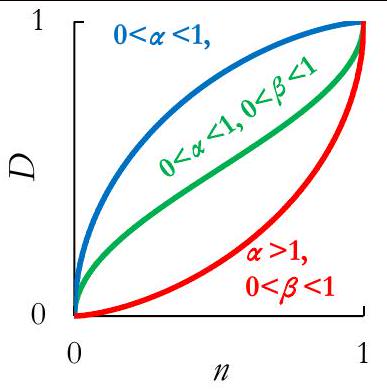
Model based on the Weibull distribution with a linear section [82]

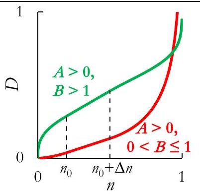
Table 9: The typical dependencies

D (n)

and

D^{'} (n)

of models based on cumulative distribution functions

Model based on the Weibull distribution. Based on the use of the Weibull cumulative distribution function, the authors [81] developed a model:

\begin{matrix} (61) & D_{E} = 1 - \frac{E_{R}}{E_{0}} = A (- \ln (1 - n))^{\frac{1}{B}} or D_{σ} = 1 - \frac{σ_{R}}{σ_{U}} = A (- \ln (1 - n))^{\frac{1}{B}}, \end{matrix}

where

A

and

B

are parameters which values depend on the loading conditions. Within this model, the damage function and its derivatives have the form:

\begin{aligned} D = A (- \ln (1 - n))^{\frac{1}{B}}, D^{'} = \frac{A}{B} (- \ln (1 - n))^{\frac{1}{B} - 1} \frac{1}{1 - n}, \\ (62) & D^{''} = \frac{A}{B} (- \ln (1 - n))^{\frac{1}{B} - 2} \frac{1}{(1 - n)^{2}} (\frac{1}{B} - 1 - \ln (1 - n)) . \end{aligned}

This model can only be used with a relative number of cycles and only with "normalized damage", since

D \to \infty

n \to 1

. The conditions for the damage function to be positive and its value to be zero at

n = 0

imply that

A > 0, B > 0

. This same condition is sufficient for the first derivative of the damage function to be positive. Depending on the value of parameter

B

, the following options are possible (Tab. 9):

when $B \leq 1$ , then $D^{''} \geq 0$ and the function is applicable to describing two-stage dependencies with accelerated damage accumulation;
when $B > 1$ , then the second derivative of the damage function changes sign, and the function is applicable to describing three-stage "fast-slow-fast" dependencies.
A drawback of the model is that it obtains values of $D > 1$ ; however, this behavior most often occurs as $n \to 1$ .
Model based on the Weibull distribution with a linear section. The authors [82] developed a modification of the previous model, consisting of adding an additional linear section that maintains the continuity and smoothness of the damage function:

\begin{matrix} (63) & D = {\begin{matrix} (1 - Δ D) A {(- \ln (1 - \frac{n}{1 - Δ n}))}^{\frac{1}{B}}, 0 \leq n < n_{0}, \\ D_{0} + (n - n_{0}) \frac{Δ D}{Δ n}, n_{0} \leq n < n_{0} + Δ n, \\ Δ D + (1 - Δ D) A {(- \ln (1 - \frac{n - Δ n}{1 - Δ n}))}^{\frac{1}{B}}, n_{0} + Δ n \leq n \leq 1, \end{matrix} \end{matrix}

where

A, B, n_{0}, Δ n

are parameters whose values depend on the loading conditions, parameters

D_{0}

and

Δ D

are determined by the expressions:

\begin{matrix} (64) & D_{0} = (1 - Δ D) A {(- \ln (1 - \frac{n_{0}}{1 - Δ n}))}^{\frac{1}{B}}, Δ D = 1 - {[1 + \frac{A}{B} {(- \ln (1 - \frac{n_{0}}{1 - Δ n}))}^{\frac{1}{B} - 1} \frac{Δ n}{1 - Δ n - n_{0}}]}^{- 1} . \end{matrix}

The necessary constraints (including those from the original model) are:

A > 0, B > 0, 0 \leq n_{0} < 1 - Δ n, 0 < Δ n < 1

. As in the original version, the model can be used only with the relative number of cycles, and also with "normalized damage". The derivatives of the damage function have the form of (Eq. 65).
Given the imposed constraints, the damage function is automatically positive. Depending on the value of parameter

B

, the following options are possible:

when $B \leq 1$ , then $D^{''} \geq 0$ and the function is applicable to describing two-stage dependencies with accelerated damage accumulation;
if $B > 1$ , then the second derivative of the damage function changes sign, and the function is applicable to describing three-stage "fast-slow-fast" dependencies.

\begin{aligned} (65) & D^{'} = {\begin{matrix} (1 - Δ D) \frac{A}{B} {(- \ln (1 - \frac{n}{1 - Δ n}))}^{\frac{1}{B} - 1} \frac{1}{1 - Δ n - n}, 0 \leq n < n_{0}, \\ \frac{Δ D}{Δ n}, n_{0} \leq n < n_{0} + Δ n, \\ (1 - Δ D) \frac{A}{B} {(- \ln (1 - \frac{n - Δ n}{1 - Δ n}))}^{\frac{1}{B} - 1} \frac{1}{1 - n}, n_{0} + Δ n \leq n \leq 1, \\ D^{''} = {\begin{matrix} (1 - Δ D) \frac{A}{B} {(- \ln (1 - \frac{n}{1 - Δ n}))}^{\frac{1}{B} - 2} \frac{1}{(1 - Δ n - n)^{2}} (\frac{1}{B} - 1 - \ln (1 - \frac{n}{1 - Δ n})), 0 \leq n < n_{0}, \\ 0, n_{0} \leq n < n_{0} + Δ n, \\ (1 - Δ D) \frac{A}{B} {(- \ln (1 - \frac{n - Δ n}{1 - Δ n}))}^{\frac{1}{B} - 2} \frac{1}{(1 - n)^{2}} (\frac{1}{B} - 1 - \ln (1 - \frac{n - Δ n}{1 - Δ n})), n_{0} + Δ n \leq n \leq 1, \end{matrix} \end{matrix} \end{aligned}

Further expansion of this class of phenomenological models for describing the residual mechanical properties of polymer composites after fatigue loadings by using various probability distribution laws appears promising.

Discussion

Summary of the results

Thus, within the framework of the developed methodology, an analysis and classification of phenomenological models of residual mechanical characteristics have been carried out. Various models have been grouped by their primary function: polynomial, power, exponential, logarithmic, and trigonometric, with a separate category for models utilizing cumulative distribution functions. Each group is further divided into subgroups according to the specific form of the function that defines the dependence of damage (or "normalized damage") on the number of loading cycles (either absolute or relative). A generalized form of the classification is presented in Tab. 10. The total number of subgroups (i.e., the total number of distinct characteristic functions) amounted to 28 . Of these, 17 functions can only use the relative number of cycles (without explicitly introducing fatigue life as an additional parameter), 4 functions can only use the absolute number of cycles (logarithmic models), and 7 functions allow both variants (due to the presence of a parameter multiplied by the number of cycles). In addition, 16 functions can only be used with "normalized damage", which requires determination of the residual value of the material property prior to fatigue failure, while the other 12 functions can be used with both definitions of damage. Twenty-four models are capable of describing two-stage dependencies with decelerated damage accumulation (without the third stage), 20 models can describe two-stage dependencies with accelerated damage accumulation (without the first stage), and 19 models are able to describe three-stage "fast-slow-fast" dependencies.

However, only 12 models can be used as universal ones that can describe all types of mechanical properties degradation curves.
The proposed classification can be used as a tool to select the model that best describes experimental data on residual mechanical characteristics. Based on the characteristic shape of the experimental curves and considering the possible exclusion of certain sections, only those models that are capable of describing the observed dependencies can be immediately selected. Furthermore, when determining the dependence of model parameters on loading conditions, the ranges of parameter values that ensure damage remains within the interval

[0; 1]

, maintain a positive rate of damage growth, and allow the description of two or three characteristic stages can be considered from the outset. In addition, the presented derivatives of the damage functions can be used to determine the boundaries of the stages of fatigue damage accumulation based on the characteristic rate of damage growth.
Concurrently, this classification provides a foundation for formulating novel phenomenological models. This can be achieved both by modernizing existing functions and by searching for new variants (for example, within the group of models based on cumulative distribution functions, only two types of distributions were used, whereas the total number of distribution functions amounts to several dozen).

Limitations

Within the developed methodology, the considered models have several limitations:

the stochastic nature of the degradation of mechanical properties is not considered. Experimental data on residual properties might demonstrate deviations from the fitting curves, which must be taken into account in the calculation of the model parameters [5, 47, 70, 73, 78];
the problem of damage accumulation under various loading conditions (including temperature changes) is not considered. However, the degradation of mechanical properties might lead to a change in the stress-strain state even under similar loading of the structure;
no possible "healing" of the material is taken into account. For example, work [83] demonstrated growth of the residual stiffness after preliminary cyclic loading, which might be caused by a local change in the reinforcement scheme. Possible directions for the development of phenomenological models are discussed below.

Table 10: Classification of the phenomenological models of residual mechanical properties

No.

Model class

Model name

Damage function

Number of parameters

Constraints for parameters

Absolute /relative number of cycles

Damage / normalized damage

Descriptive capability

2-stage,

D^{''} \geq 0

2-stage,

D^{''} \leq 0

3-stage

Wang C., Zhang J.

D = B - A \ln (\frac{C - n}{n})

A > 0, C > 1

B - A \ln (C - 1) \leq 1

- / +

+ / +

C \geq 2

1 < C < 2

Whitworth H.A.

D = 1 - [1 - A \ln (1 + N)]^{B}

A \neq 0, A < 1 / \ln (1 + N_{A})

+ / -

+ / +

B < 0 or B \geq 1 +

Logarithmic models

Ramakrishnan V., Jayaraman N.

D = A \ln (N + 1) + B N - C \ln (1 - \frac{N}{N_{f}})

A > 0, B > 0, C > 0

A \ln (N_{f}) + B (N_{f} - 1) + + Cln (N_{ℓ}) \leq 1

+ / -

+ / +

C / N_{f}^{2} \geq A

C \leq A / N_{f}^{2}

C / N_{f}^{2} < A

C > A / N_{f}^{2}

Adam T., Dickson R.F., Jones C.J., Reiter H., Harris B.

D = 1 - {(1 - {(\frac{\ln 2 N}{\ln 2 N_{f}})}^{A})}^{B}

A > 0, B > 0

+ / -

- / +

Trigonometric models

Yao W.X., Himmel N.

D = \frac{\sin (A n) \cos (A - B)}{\sin (A) \cos (A n - B)}

0 < A < π

- π / 2 < B < π / 2

(A - B) < π / 2

- / +

B < 0

A < B

B > 0, A > B

Gao J., Zhu P., Yuan Y., Wu Z., Xu R.

D = \frac{\sin (△ n) \cos (B)}{\sin (A) \cos (B n^{A})}

0 < A < π

- π / 2 < B < π / 2

, (

B n^{4 - 1} - - 1) \sin (A n) \sin (B n^{4}) + + \cos (A n) \cos (B n^{- 1}) > 0

- / +

Liu H., Zhang Z., Jia H., Liu Y., Leng J.

D = \cos (\frac{π}{2} {(1 - n^{B})}^{- A})

D = 1 - \sin (\frac{π}{2} {(1 - n^{B})}^{A})

A > 0, B > 0

- / +

0 < A \leq 0.5

B \geq 1

A \geq 0.5

0 < B < 1

, or

A \geq 1, B = 1

0 < A < 0.5

0 < B < 1

A > 0, B > 0

- / +

0 < A < 1

B \geq 0.5

, or

A = 1, B \geq 1

A \geq 1

0 < B \leq 0.5

0 < A < 1

0 < B < 0.5

Models based on the cumulative distribution

distribution functions

Based on betadistribution

D = \frac{B_{n} (α, β)}{B (α, β)}

a > 0, a \neq 1

β > 0, β \neq 1

- / +

a > 1, β < 1

a < 1, β > 1

a < 1, β < 1

Based on Weibull distribution

D = A (- \ln (1 - n))^{\frac{1}{B}}

A > 0, B > 0

- / +

B \leq 1

B > 1

Based on Weibull distribution with a linear section

D = {\begin{matrix} (1 - Δ D) A {(- \ln (1 - \frac{n}{1 - Δ n}))}^{\frac{1}{B}}, 0 \leq n < n_{0} \\ D_{0} + (n - n_{0}) \frac{Δ D}{Δ n}, n_{0} \leq n < n_{0} + Δ n \\ Δ D + (1 - Δ D) A {(- \ln (1 - \frac{n - Δ n}{1 - Δ n}))}^{\frac{1}{B}}, n_{0} + Δ n \leq n \leq 1 \end{matrix}

\begin{matrix} A > 0, B > 0, \\ 0 \leq n_{0} < 1 - Δ n, \\ 0 < Δ n < 1 \end{matrix}

- / +

B \leq 1

B > 1

*The descriptive capability is proved by parameters variation

**The simplified version of the model is analyzed

No. Model class Model name Damage function Number of parameters Constraints for parameters Absolute /relative number of cycles Damage / normalized damage Descriptive capability 2-stage, D^('') >= 0 2-stage, D^('') <= 0 3-stage 18 Wang C., Zhang J. D=B-A ln((C-n)/(n)) 3 A > 0,C > 1, B-A ln(C-1) <= 1 - / + + / + - + C >= 2 + 1 < C < 2 19 Whitworth H.A. D=1-[1-A ln(1+N)]^(B) 2 A!=0,A < 1//ln(1+N_(A)) + / - + / + - + B < 0" or "B >= 1+ + 20 Logarithmic models Ramakrishnan V., Jayaraman N. D=A ln(N+1)+BN-C ln(1-(N)/(N_(f))) 4 A > 0,B > 0,C > 0, A ln(N_(f))+B(N_(f)-1)++Cln(N_(ℓ)) <= 1 + / - + / + + C//N_(f)^(2) >= A + C <= A//N_(f)^(2) + C//N_(f)^(2) < A, C > A//N_(f)^(2) 21 Adam T., Dickson R.F., Jones C.J., Reiter H., Harris B. D=1-(1-((ln 2N)/(ln 2N_(f)))^(A))^(B) 3 A > 0,B > 0 + / - - / + - +* +* 22 Trigonometric models Yao W.X., Himmel N. D=(sin(An)cos(A-B))/(sin(A)cos(An-B)) 2 0 < A < pi, -pi//2 0,A > B 23 Gao J., Zhu P., Yuan Y., Wu Z., Xu R. D=(sin(/_\n)cos(B))/(sin(A)cos(Bn^(A))) 2 0 < A < pi, -pi//2 0 - / + - / + +* +* +* 24 "Liu H., Zhang Z., Jia H., Liu Y., Leng J. D=cos((pi)/(2)(1-n^(B))^(-A)) D=1-sin((pi)/(2)(1-n^(B))^(A))" 2 A > 0,B > 0 - / + - / + + 0 < A <= 0.5, B >= 1 + A >= 0.5, 0 = 1,B=1 + 0 < A < 0.5, 0 0,B > 0 - / + - / + + 0 < A < 1, B >= 0.5, or A=1,B >= 1 + A >= 1, 0 0,a!=1, beta > 0,beta!=1 - / + - / + + a > 1,beta < 1 + a < 1,beta > 1 + a < 1,beta < 1 27 https://cdn.mathpix.com/cropped/ade2f789-5a59-4962-b074-849fdd5f4a97-30.jpg?height=55&width=30&top_left_y=2437&top_left_x=1559 Based on Weibull distribution D=A(-ln(1-n))^((1)/(B)) 2 A > 0,B > 0 - / + - / + + B <= 1 - + B > 1 Based on Weibull distribution with a linear section D={[(1-Delta D)A(-ln(1-(n)/(1-Delta n)))^((1)/(B))","0 <= n < n_(0)],[D_(0)+(n-n_(0))(Delta D)/(Delta n)","n_(0) <= n < n_(0)+Delta n],[Delta D+(1-Delta D)A(-ln(1-(n-Delta n)/(1-Delta n)))^((1)/(B))","quadn_(0)+Delta n <= n <= 1]:} 4 "A > 0,B > 0, 0 <= n_(0) < 1-Delta n, 0 < Delta n < 1" - / + - / + + B <= 1 - + B > 1 *The descriptive capability is proved by parameters variation **The simplified version of the model is analyzed

| No. | | Model class | Model name | Damage function | Number of parameters | Constraints for parameters | Absolute /relative number of cycles | Damage / normalized damage | Descriptive capability | | | | :--- | :--- | :--- | :--- | :--- | :--- | :--- | :--- | :--- | :--- | :--- | :--- | | | | 2-stage, $D^{\prime \prime} \geq 0$ | | | | | | | 2-stage, $D^{\prime \prime} \leq 0$ | 3-stage | | 18 | | | | Wang C., Zhang J. | $D=B-A \ln \left(\frac{C-n}{n}\right)$ | 3 | $A>0, C>1$, $B-A \ln (C-1) \leq 1$ | - / + | + / + | - | + $C \geq 2$ | + $1<C<2$ | | 19 | | | Whitworth H.A. | $D=1-[1-A \ln (1+N)]^{B}$ | 2 | $A \neq 0, A<1 / \ln \left(1+N_{A}\right)$ | + / - | + / + | - | + $B<0 \text { or } B \geq 1+$ + | | | 20 | | Logarithmic models | Ramakrishnan V., Jayaraman N. | $D=A \ln (N+1)+B N-C \ln \left(1-\frac{N}{N_{f}}\right)$ | 4 | $A>0, B>0, C>0$, $A \ln \left(N_{f}\right)+B\left(N_{f}-1\right)+ +\operatorname{Cln}\left(N_{\ell}\right) \leq 1$ | + / - | + / + | + $C / N_{f}^{2} \geq A$ | + $C \leq A / N_{f}^{2}$ | + $C / N_{f}^{2}<A$, $C>A / N_{f}^{2}$ | | 21 | | | Adam T., Dickson R.F., Jones C.J., Reiter H., Harris B. | $D=1-\left(1-\left(\frac{\ln 2 N}{\ln 2 N_{f}}\right)^{A}\right)^{B}$ | 3 | $A>0, B>0$ | + / - | - / + | - | +* | +* | | 22 | | Trigonometric models | Yao W.X., Himmel N. | $D=\frac{\sin (A n) \cos (A-B)}{\sin (A) \cos (A n-B)}$ | 2 | $0<A<\pi$, $-\pi / 2<B<\pi / 2$, $(A-B)<\pi / 2$ | - / + | - / + | + $B<0$ | + $A<B$ | + $B>0, A>B$ | | 23 | | | Gao J., Zhu P., Yuan Y., Wu Z., Xu R. | $D=\frac{\sin (\triangle n) \cos (B)}{\sin (A) \cos \left(B n^{A}\right)}$ | 2 | $0<A<\pi$, $-\pi / 2<B<\pi / 2$, ( $B n^{4-1}- -1) \sin (A n) \sin \left(B n^{4}\right)+ +\cos (A n) \cos \left(B n^{-1}\right)>0$ | - / + | - / + | +* | +* | +* | | 24 | | | Liu H., Zhang Z., Jia H., Liu Y., Leng J. $D=\cos \left(\frac{\pi}{2}\left(1-n^{B}\right)^{-A}\right)$ $D=1-\sin \left(\frac{\pi}{2}\left(1-n^{B}\right)^{A}\right)$ | | 2 | $A>0, B>0$ | - / + | - / + | + $0<A \leq 0.5$, $B \geq 1$ | + $A \geq 0.5$, $0<B<1$, or $A \geq 1, B=1$ | + $0<A<0.5$, $0<B<1$ | | 25 | | | | | 2 | $A>0, B>0$ | - / + | - / + | + $0<A<1$, $B \geq 0.5$, or $A=1, B \geq 1$ | + $A \geq 1$, $0 distribution functions | Based on betadistribution | $D=\frac{B_{n}(\alpha, \beta)}{B(\alpha, \beta)}$ | 2 | $a>0, a \neq 1$, $\beta>0, \beta \neq 1$ | - / + | - / + | + $a>1, \beta<1$ | + $a<1, \beta>1$ | + $a<1, \beta<1$ | | 27 | ![](https://cdn.mathpix.com/cropped/ade2f789-5a59-4962-b074-849fdd5f4a97-30.jpg?height=55&width=30&top_left_y=2437&top_left_x=1559) | | Based on Weibull distribution | $D=A(-\ln (1-n))^{\frac{1}{B}}$ | 2 | $A>0, B>0$ | - / + | - / + | + $B \leq 1$ | - | + $B>1$ | | | | | Based on Weibull distribution with a linear section | $D=\left\{\begin{array}{c} (1-\Delta D) A\left(-\ln \left(1-\frac{n}{1-\Delta n}\right)\right)^{\frac{1}{B}}, 0 \leq n<n_{0} \\ D_{0}+\left(n-n_{0}\right) \frac{\Delta D}{\Delta n}, n_{0} \leq n<n_{0}+\Delta n \\ \Delta D+(1-\Delta D) A\left(-\ln \left(1-\frac{n-\Delta n}{1-\Delta n}\right)\right)^{\frac{1}{B}}, \quad n_{0}+\Delta n \leq n \leq 1 \end{array}\right.$ | 4 | $\begin{gathered} A>0, B>0, \\ 0 \leq n_{0}<1-\Delta n, \\ 0<\Delta n<1 \end{gathered}$ | - / + | - / + | + $B \leq 1$ | - | + $B>1$ | | *The descriptive capability is proved by parameters variation | | | | | | | | | | | | | **The simplified version of the model is analyzed | | | | | | | | | | | |

Table 10: Classification of the phenomenological models of residual mechanical properties

Future scopes

Based on the review, several promising directions for the further development of phenomenological models of residual mechanical characteristics can also be identified.
The first direction is related to the introduction of stochasticity in the distribution of the material's elastic and strength characteristics into the models. Such approaches have been proposed in works

[29, 30, 39, 40, 44, 45, 47, 49 - 53, 55, 56, 59

, 71], with the Weibull distribution law being the most frequently used. The necessity of this line of development is determined by the presence (in some cases significant) of scatter in the mechanical properties of polymer composites.
The second direction concerns the application of the considered models to the problem of damage summation under variable loading conditions. This direction has been addressed in papers [28, 38, 78, 79, 80] (Tab. 11). The change in residual strength under multiple damage levels was considered in works

[12, 36, 44, 45, 49, 50, 54, 66, 67, 84]

(Tab. 12). The relevance of this direction is justified by the fact that fatigue damage accumulation rarely occurs under constant loading conditions. Moreover, changes in the mechanical characteristics themselves can lead to alterations in the stress-strain state within the cycle.

No	Authors	Model
Damage accumulation under the variable amplitude fatigue loading
1	Owen M. J., Howe R. J. 1972 [38]	$\sum D_{σ} = \sum [B n_{i} - A n_{i}^{2}]$
2	Wu F., Yao W.X. 2010 [28]	$D (n_{i}) = 1 - {[1 - {(\frac{N_{i} + N_{i, i - 1}}{N_{f_{i}}})}^{B_{i}}]}^{A_{i}}, N_{i, i - 1} = N_{f_{i}} {[1 - {(1 - {(\frac{N_{i - 1} + N_{i - 1, i - 2}}{N_{f_{i - 1}}})}^{B_{i - 1}})}^{\frac{A_{i - 1}}{A_{i}}}]}^{1 / B_{i}}$
3	Shiri S., Yazdani M., Pourgol-Mohammad M. 2015 [78]	$\begin{matrix} D (n_{i}) = {(\frac{N_{i} + N_{i, i - 1}^{\frac{\log σ_{max_{i}}}{\log σ_{max_{i - 1}}}}}{N_{f_{i}}})}^{\frac{A_{w} (1 - R)}{B_{w}}}, N_{i, i - 1} = N_{f_{i}} {(\frac{\sin (A_{i - 1} n_{i - 1}) \cos (A_{i - 1} - B_{i - 1})}{\sin (A_{i - 1}) \cos (A_{i - 1} n_{i - 1} - B_{i - 1})})}^{\frac{B_{w}}{A_{w} (1 - R)}}, \\ B_{w} = \frac{σ_{min}}{σ_{max}} \sqrt{B_{i - 1} + B_{i}}, A_{w} = \sqrt{A_{i - 1} + A_{i}} \end{matrix}$
4	Gao J., Zhu P., Yuan Y., Wu Z., Xu R. 2022 [79]	$D_{i} (n_{i}) = \frac{\sin (A_{i} \frac{N_{i}}{N_{f_{i}}}) \cos (B_{i})}{\sin (A_{i}) \cos [B_{i} {(\frac{N_{i}}{N_{f_{i}}})}^{A_{i}}]}, D_{i - 1} (n_{i - 1}) = \frac{\sin (A_{i - 1} \frac{N_{i - 1}}{N_{f_{i - 1}}}) \cos (B_{i - 1})}{\sin (A_{i - 1}) \cos [B_{i - 1} {(\frac{N_{i - 1}}{N_{f_{i - 1}}})}^{A_{i - 1}}]}$
5	Liu H., Zhang Z., Jia H., Liu Y., Leng J. 2020 [80]	$D (n_{i}) = 1 - \sin (\frac{π}{2} {(1 - {(\frac{N_{i} + N_{i, i - 1}}{N_{f_{i}}})}^{B_{i}})}^{A_{i}}), N_{i, i - 1} = N_{f_{i}} {(1 - {(1 - {(\frac{N_{i - 1} + N_{i - 1, i - 2}}{N_{f_{i - 1}}})}^{B_{i - 1}})}^{\frac{A_{i - 1}}{A_{i}}})}^{\frac{1}{B_{i}}}$
Table 11: Damage accumulation in the considered models
No	Authors	Model
Residual strength models for several stress levels
1	Broutman L. J., Sahu S. 1972 [36]	$σ_{R_{1} (n_{1})} = σ_{U} - (σ_{U} - σ_{{max}_{1}}) n_{1}, σ_{R_{2} (n_{1} + n_{2})} = σ_{R_{1}} - (σ_{U} - σ_{{max}_{2}}) n_{2}$ $σ_{R_{2} (n_{1} + n_{2})} = σ_{U} - (σ_{U} - σ_{max_{1}}) n_{1} - (σ_{U} - σ_{max_{2}}) n_{2}$
2	Shaff J. R., Davidson B. D. 1997 [44, 45]	$σ_{R} (\sum_{i = 1}^{j} N_{i}) = σ_{U} - (σ_{U} - σ_{max_{j}}) {[\frac{N_{e f f_{j}} + N_{j}}{N_{f_{j}}}]}^{A_{j}}, N_{e f f_{j}} = {[\frac{σ_{U} - σ_{R} (\sum_{i = 1}^{j - 1} N_{i})}{σ_{U} - σ_{max_{j}}}]}^{\frac{1}{A_{j}}} N_{j}$

| No | Authors | Model | | :--- | :--- | :--- | | Damage accumulation under the variable amplitude fatigue loading | | | | 1 | Owen M. J., Howe R. J. 1972 [38] | $\sum D_{\sigma}=\sum\left[B n_{i}-A n_{i}{ }^{2}\right]$ | | 2 | Wu F., Yao W.X. 2010 [28] | $D\left(n_{i}\right)=1-\left[1-\left(\frac{N_{i}+N_{i, i-1}}{N_{f_{i}}}\right)^{B_{i}}\right]^{A_{i}}, \quad N_{i, i-1}=N_{f_{i}}\left[1-\left(1-\left(\frac{N_{i-1}+N_{i-1, i-2}}{N_{f_{i-1}}}\right)^{B_{i-1}}\right)^{\frac{A_{i-1}}{A_{i}}}\right]^{1 / B_{i}}$ | | 3 | Shiri S., Yazdani M., Pourgol-Mohammad M. 2015 [78] | $\begin{gathered} D\left(n_{i}\right)=\left(\frac{N_{i}+N_{i, i-1}^{\frac{\log \sigma_{\max _{i}}}{\log \sigma_{\max _{i-1}}}}}{N_{f_{i}}}\right)^{\frac{A_{w}(1-R)}{B_{w}}}, \quad N_{i, i-1}=N_{f_{i}}\left(\frac{\sin \left(A_{i-1} n_{i-1}\right) \cos \left(A_{i-1}-B_{i-1}\right)}{\sin \left(A_{i-1}\right) \cos \left(A_{i-1} n_{i-1}-B_{i-1}\right)}\right)^{\frac{B_{w}}{A_{w}(1-R)}}, \\ B_{w}=\frac{\sigma_{\text {min }}}{\sigma_{\text {max }}} \sqrt{B_{i-1}+B_{i}}, \quad A_{w}=\sqrt{A_{i-1}+A_{i}} \end{gathered}$ | | 4 | Gao J., Zhu P., Yuan Y., Wu Z., Xu R. 2022 [79] | $D_{i}\left(n_{i}\right)=\frac{\sin \left(A_{i} \frac{N_{i}}{N_{f_{i}}}\right) \cos \left(B_{i}\right)}{\sin \left(A_{i}\right) \cos \left[B_{i}\left(\frac{N_{i}}{N_{f_{i}}}\right)^{A_{i}}\right]}, D_{i-1}\left(n_{i-1}\right)=\frac{\sin \left(A_{i-1} \frac{N_{i-1}}{N_{f_{i-1}}}\right) \cos \left(B_{i-1}\right)}{\sin \left(A_{i-1}\right) \cos \left[B_{i-1}\left(\frac{N_{i-1}}{N_{f_{i-1}}}\right)^{A_{i-1}}\right]}$ | | 5 | Liu H., Zhang Z., Jia H., Liu Y., Leng J. 2020 [80] | $D\left(n_{i}\right)=1-\sin \left(\frac{\pi}{2}\left(1-\left(\frac{N_{i}+N_{i, i-1}}{N_{f_{i}}}\right)^{B_{i}}\right)^{A_{i}}\right), \quad N_{i, i-1}=N_{f_{i}}\left(1-\left(1-\left(\frac{N_{i-1}+N_{i-1, i-2}}{N_{f_{i-1}}}\right)^{B_{i-1}}\right)^{\frac{A_{i-1}}{A_{i}}}\right)^{\frac{1}{B_{i}}}$ | | Table 11: Damage accumulation in the considered models | | | | No | Authors | Model | | Residual strength models for several stress levels | | | | 1 | Broutman L. J., Sahu S. 1972 [36] | $\sigma_{R_{1}\left(n_{1}\right)}=\sigma_{U}-\left(\sigma_{U}-\sigma_{\text {max }_{1}}\right) n_{1}, \quad \sigma_{R_{2}\left(n_{1}+n_{2}\right)}=\sigma_{R_{1}}-\left(\sigma_{U}-\sigma_{\text {max }_{2}}\right) n_{2}$ $\sigma_{R_{2}\left(n_{1}+n_{2}\right)}=\sigma_{U}-\left(\sigma_{U}-\sigma_{\max _{1}}\right) n_{1}-\left(\sigma_{U}-\sigma_{\max _{2}}\right) n_{2}$ | | 2 | Shaff J. R., Davidson B. D. 1997 [44, 45] | $\sigma_{R}\left(\sum_{i=1}^{j} N_{i}\right)=\sigma_{U}-\left(\sigma_{U}-\sigma_{\max _{j}}\right)\left[\frac{N_{e f f_{j}}+N_{j}}{N_{f_{j}}}\right]^{A_{j}}, \quad N_{e f f_{j}}=\left[\frac{\sigma_{U}-\sigma_{R}\left(\sum_{i=1}^{j-1} N_{i}\right)}{\sigma_{U}-\sigma_{\max _{j}}}\right]^{\frac{1}{A_{j}}} N_{j}$ |

Epaarachchi J.A., Clausen P.D. 2003, 2005 [49, 50]

σ_{R (i)} = σ_{R (i - 1)} - \frac{A}{f^{C}} {(\frac{σ_{max}}{σ_{R (i - 1)}})}^{0.6 - B | \sin θ |} [σ_{max} (1 - B)^{1.6 - B | \sin θ |}] (N^{C} - 1) α_{i}, α_{i} = 1 - {[1 - {(\frac{N}{N_{R (i)}})}^{C}]}^{C}

where

f

- the frequency,

θ

- the smallest ply angle of the laminate to the loading direction,

B = R

- stress ratio for

- \infty \leq R \leq 1, B = 1 / R

for

1 < R \leq \infty

α_{i} -

a 'factor' that accounts for the fraction of strength degraded under variable amplitude loading,

N_{R (i)}

- the residual life at

σ_{max}

after the loading at the (

i - 1

)th step.

Hashin Z. 1985 [54]

\begin{matrix} σ_{R_{1} (n_{1})}^{A} = σ_{U}^{A} - (σ_{U}^{A} - σ_{{max}_{1}}^{A}) n_{1}, σ_{R_{2} (n_{1} + n_{2})}^{A} = σ_{R_{1}}^{A} - (σ_{U}^{A} - σ_{{max}_{2}}^{A}) n_{2}, \\ σ_{R_{2} (n_{1} + n_{2})}^{A} = σ_{U}^{A} - (σ_{U}^{A} - σ_{{max}_{1}}^{A}) n_{1} - (σ_{U}^{A} - σ_{{max}_{2}}^{A}) n_{2} \end{matrix}

Post N. L., Case S. W., Lesko J. J. 2008 [12]

σ_{R_{i}}^{A_{i}} = σ_{U}^{A_{i}} - (σ_{U}^{A_{i}} - σ_{max_{i}}^{A_{i}}) {(\frac{N_{i} + N_{e q_{i - 1}}}{N_{f_{i}}})}^{B_{i}}, N_{e q_{i - 1}} = {[\frac{σ_{U}^{A_{i}} - σ_{R_{i - 1}}^{A_{i}}}{σ_{U}^{A_{i}} - σ_{max_{i}}^{A_{i}}}]}^{\frac{1}{B_{i}}} N_{f_{i}}

Kassapoglou, C. 2010, 2011 [66, 67]

σ_{R_{1}} = {(σ_{max_{1}})}^{\frac{N_{1}}{N_{f 1} - 1}} {(σ_{U})}^{\frac{N_{f 1} - N_{1} - 1}{N_{f 1} - 1}}, σ_{R_{2}} = {(σ_{max_{2}})}^{\frac{N_{2}}{N_{f 2} - 1} + \frac{N_{1}}{N_{f 1} - 1} \ln (N_{f 2})} {(σ_{U})}^{1 - (\frac{N_{2}}{N_{f 2} - 1} + \frac{N_{1}}{N_{f 1} - 1} - \frac{\ln (N_{f 1})}{\ln (N_{f 2})})}

the residual strength after the first two segments,

N_{1}

σ_{max 1}

followed by

N_{2}

σ_{max 2}

Passipoularidis V. A., Philippidis T. P 2009 [84]

σ_{R_{i}} = σ_{U} - (σ_{U} - σ_{{max}_{i}}) {(\frac{N_{i} + N_{e q_{i}}}{N_{f_{i}}})}^{A \exp (B \frac{N_{i} + N_{q_{i}}}{N_{f_{i}}})}, N_{e q_{i}} = {[1 - {(\frac{σ_{R_{i - 1}} - σ_{{max}_{i}}}{σ_{U} - σ_{{max}_{i}}})}^{Y}]}^{\frac{1}{V}} N_{f_{i}},

where

n_{eq}

- the number of constant amplitude fatigue cycles that would have brought the strength down to

σ_{R_{i - 1}}

3 Epaarachchi J.A., Clausen P.D. 2003, 2005 [49, 50] sigma_(R(i))=sigma_(R(i-1))-(A)/(f^(C))((sigma_("max "))/(sigma_(R(i-1))))^(0.6-B|sin theta|)[sigma_("max ")(1-B)^(1.6-B|sin theta|)](N^(C)-1)alpha_(i),quadalpha_(i)=1-[1-((N)/(N_(R(i))))^(C)]^(C) where f - the frequency, theta - the smallest ply angle of the laminate to the loading direction, B=R - stress ratio for -oo <= R <= 1,B=1//R for 1 < R <= oo, alpha_(i)- a 'factor' that accounts for the fraction of strength degraded under variable amplitude loading, N_(R(i)) - the residual life at sigma_("max ") after the loading at the ( i-1 )th step. 4 Hashin Z. 1985 [54] "sigma_(R_(1)(n_(1)))^(A)=sigma_(U)^(A)-(sigma_(U)^(A)-sigma_(max _(1))^(A))n_(1),quadsigma_(R_(2)(n_(1)+n_(2)))^(A)=sigma_(R_(1))^(A)-(sigma_(U)^(A)-sigma_(max _(2))^(A))n_(2), sigma_(R_(2)(n_(1)+n_(2)))^(A)=sigma_(U)^(A)-(sigma_(U)^(A)-sigma_(max _(1))^(A))n_(1)-(sigma_(U)^(A)-sigma_(max _(2))^(A))n_(2)" 5 Post N. L., Case S. W., Lesko J. J. 2008 [12] sigma_(R_(i))^(A_(i))=sigma_(U)^(A_(i))-(sigma_(U)^(A_(i))-sigma_(max_(i))^(A_(i)))((N_(i)+N_(eq_(i-1)))/(N_(f_(i))))^(B_(i)),quadN_(eq_(i-1))=[(sigma_(U)^(A_(i))-sigma_(R_(i-1))^(A_(i)))/(sigma_(U)^(A_(i))-sigma_(max_(i))^(A_(i)))]^((1)/(B_(i)))N_(f_(i)) 6 Kassapoglou, C. 2010, 2011 [66, 67] "sigma_(R_(1))=(sigma_(max_(1)))^((N_(1))/(N_(f1)-1))(sigma_(U))^((N_(f1)-N_(1)-1)/(N_(f1)-1)),quadsigma_(R_(2))=(sigma_(max_(2)))^((N_(2))/(N_(f2)-1)+(N_(1))/(N_(f1)-1)ln(N_(f2)))(sigma_(U))^(1-((N_(2))/(N_(f2)-1)+(N_(1))/(N_(f1)-1)-(ln(N_(f1)))/(ln(N_(f2))))) the residual strength after the first two segments, N_(1) at sigma_(max1) followed by N_(2) at sigma_(max2)" 7 Passipoularidis V. A., Philippidis T. P 2009 [84] "sigma_(R_(i))=sigma_(U)-(sigma_(U)-sigma_("max "_(i)))((N_(i)+N_(eq_(i)))/(N_(f_(i))))^(A exp(B(N_(i)+N_(q_(i)))/(N_(f_(i))))),quadN_(eq_(i))=[1-((sigma_(R_(i-1))-sigma_("max "_(i)))/(sigma_(U)-sigma_("max "_(i))))^(Y)]^((1)/(V))N_(f_(i)), where n_("eq ") - the number of constant amplitude fatigue cycles that would have brought the strength down to sigma_(R_(i-1))"

| 3 | Epaarachchi J.A., Clausen P.D. 2003, 2005 [49, 50] | $\sigma_{R(i)}=\sigma_{R(i-1)}-\frac{A}{f^{C}}\left(\frac{\sigma_{\text {max }}}{\sigma_{R(i-1)}}\right)^{0.6-B\|\sin \theta\|}\left[\sigma_{\text {max }}(1-B)^{1.6-B\|\sin \theta\|}\right]\left(N^{C}-1\right) \alpha_{i}, \quad \alpha_{i}=1-\left[1-\left(\frac{N}{N_{R(i)}}\right)^{C}\right]^{C}$ where $f$ - the frequency, $\theta$ - the smallest ply angle of the laminate to the loading direction, $B=R$ - stress ratio for $-\infty \leq R \leq 1, B=1 / R$ for $1<R \leq \infty$, $\alpha_{i}-$ a 'factor' that accounts for the fraction of strength degraded under variable amplitude loading, $N_{R(i)}$ - the residual life at $\sigma_{\text {max }}$ after the loading at the ( $i-1$ )th step. | | :--- | :--- | :--- | | 4 | Hashin Z. 1985 [54] | $\begin{gathered} \sigma_{R_{1}\left(n_{1}\right)}^{A}=\sigma_{U}^{A}-\left(\sigma_{U}^{A}-\sigma_{\text {max }_{1}}^{A}\right) n_{1}, \quad \sigma_{R_{2}\left(n_{1}+n_{2}\right)}^{A}=\sigma_{R_{1}}^{A}-\left(\sigma_{U}^{A}-\sigma_{\text {max }_{2}}^{A}\right) n_{2}, \\ \sigma_{R_{2}\left(n_{1}+n_{2}\right)}^{A}=\sigma_{U}^{A}-\left(\sigma_{U}^{A}-\sigma_{\text {max }_{1}}^{A}\right) n_{1}-\left(\sigma_{U}^{A}-\sigma_{\text {max }_{2}}^{A}\right) n_{2} \end{gathered}$ | | 5 | Post N. L., Case S. W., Lesko J. J. 2008 [12] | $\sigma_{R_{i}}^{A_{i}}=\sigma_{U}^{A_{i}}-\left(\sigma_{U}^{A_{i}}-\sigma_{\max _{i}}^{A_{i}}\right)\left(\frac{N_{i}+N_{e q_{i-1}}}{N_{f_{i}}}\right)^{B_{i}}, \quad N_{e q_{i-1}}=\left[\frac{\sigma_{U}^{A_{i}}-\sigma_{R_{i-1}}^{A_{i}}}{\sigma_{U}^{A_{i}}-\sigma_{\max _{i}}^{A_{i}}}\right]^{\frac{1}{B_{i}}} N_{f_{i}}$ | | 6 | Kassapoglou, C. 2010, 2011 [66, 67] | $\sigma_{R_{1}}=\left(\sigma_{\max _{1}}\right)^{\frac{N_{1}}{N_{f 1}-1}}\left(\sigma_{U}\right)^{\frac{N_{f 1}-N_{1}-1}{N_{f 1}-1}}, \quad \sigma_{R_{2}}=\left(\sigma_{\max _{2}}\right)^{\frac{N_{2}}{N_{f 2}-1}+\frac{N_{1}}{N_{f 1}-1} \ln \left(N_{f 2}\right)}\left(\sigma_{U}\right)^{1-\left(\frac{N_{2}}{N_{f 2}-1}+\frac{N_{1}}{N_{f 1}-1}-\frac{\ln \left(N_{f 1}\right)}{\ln \left(N_{f 2}\right)}\right)}$ the residual strength after the first two segments, $N_{1}$ at $\sigma_{\max 1}$ followed by $N_{2}$ at $\sigma_{\max 2}$ | | 7 | Passipoularidis V. A., Philippidis T. P 2009 [84] | $\sigma_{R_{i}}=\sigma_{U}-\left(\sigma_{U}-\sigma_{\text {max }_{i}}\right)\left(\frac{N_{i}+N_{e q_{i}}}{N_{f_{i}}}\right)^{A \exp \left(B \frac{N_{i}+N_{q_{i}}}{N_{f_{i}}}\right)}, \quad N_{e q_{i}}=\left[1-\left(\frac{\sigma_{R_{i-1}}-\sigma_{\text {max }_{i}}}{\sigma_{U}-\sigma_{\text {max }_{i}}}\right)^{Y}\right]^{\frac{1}{V}} N_{f_{i}},$ where $n_{\text {eq }}$ - the number of constant amplitude fatigue cycles that would have brought the strength down to $\sigma_{\mathrm{R}_{i-1}}$ |

Table 12: Change in residual strength under multiple damage levels.

The third direction is linked to the anisotropy of polymer composites, in particular, with the possible influence of cyclic loading along one axis on the entire spectrum of the material's elastic and strength characteristics. This direction has been highlighted in the studies [21, 27, 41, 63, 75, 85, 86]. Solving these issues will contribute to the development of strength criteria for anisotropic materials that explicitly consider the number of loading cycles.
A possible direction for further development is the reduction of the number of constraints used in the methodology for model analysis. Firstly, this involves consideration of possible "healing" effects during fatigue damage accumulation, which can be implemented by enabling of a negative value of the damage function derivative within a certain range of cycles. In addition, it appears promising to consider the existence of ranges in which the material is insensitive to cyclic loading. Cases where random initial damage of the material is taken into account

(D (0) > 0

) can also be examined, which would partially correspond to accounting for the statistical scatter of strength and deformation characteristics of the undamaged material. Moreover, the models can be adapted to analyze the structural elements as a whole [87] and take into account cyclic temperature changes [88].
It should be noted that the models considered can be used to predict the residual fatigue life of composite structures based on known current values of the material properties [30, 42, 46-48, 55, 63, 80, 89]. Furthermore, the prospects for applying phenomenological models of residual mechanical characteristics are linked to the feasibility of implementing them in strength calculations of real structures to ensure their reliability and safety. This requires boundary value problem formulations that account for the processes of fatigue damage accumulation. One such formulation was presented in work [90] based on a structural-phenomenological approach, which considered: the multi-level nature of damage accumulation processes, changes in the elastic and strength properties of the material under cyclic loading, the existence of characteristic sizes of the damage zone (i.e., non-locality of damage accumulation processes), failure due to the intersection of the loading path with the strength surface, stochastic distribution of mechanical characteristics throughout the body volume, and the influence of loading systems. This will make it possible to implement the considered models in numerical methods for solving boundary value problems, particularly in the finite element method [7,21,41,83,85,91,92].

Conclusions

Thus, the present work has carried out an analysis and classification of phenomenological models used to describe the dependencies of the residual mechanical characteristics of polymer composites subjected to cyclic loading. Within the framework of the developed methodology, the following assumptions were adopted: the constancy of
loading conditions during cyclic exposure, the absence of material "healing" under cyclic loading, and the possibility of explicitly expressing the dependence of damage on the number of loading cycles. Constraints were introduced on the range of values of the damage function and on the positivity of its first derivative, on the basis of which the admissible values of the model parameters are determined. Based on the analysis of the second derivative of the damage function, conclusions were drawn regarding the ability of the models to describe two-stage and three-stage dependencies of residual properties on the number of loading cycles. The phenomenological models presented in the literature have been classified according to the primary function employed into polynomial, power, exponential, logarithmic, and trigonometric models, as well as models based on cumulative distribution functions. Twenty-eight subgroups (i.e., distinct characteristic functions) have been outlined. Only twelve models can be used as universal ones, being able to approximate both types of two-stage dependencies and three-stage dependencies. The limitations of the present study have been outlined, and the main directions for the further development of phenomenological models have been identified.
Based on the above, it can be concluded that research into the influence of fatigue damage on the residual mechanical characteristics of polymer composites is highly relevant.

Acknowledgements

r

he study was supported by grant No. 25-79-10194 from the Russian Science Foundation, https://rscf.ru/project/25-79-10194/.

LIST OF SYMBOLS

φ_{(a),} a \in [1; k]

- set of cyclic loading parameters

P̸ (β), β \in [1; l]

- set of mechanical characteristics of a material

g_{(β)}

- functions, the number of which corresponds to the number of mechanical characteristics of the material

a_{(β)}, b_{(β)}, c_{(β)}

- parameters included in the function

g_{(β)}

K_{(β)}, β \in [1; Ω]

- integrity functions, reflecting the change in the

{p̸}_{(β)}

(integrity normalized by the initial value of the mechanical property)

D_{(β)}, β \in [1;]̸

- damage functions, reflecting the change in the

{p̸}_{(β)}

(damage normalized by the initial value of the mechanical property)

K^{*}_{(β)}

- "normalized integrity" (integrity normalized by the initial and final values of the mechanical properties)

D^{*}_{(β)}

- "normalized damage" (damage normalized by the initial and final values of the mechanical properties)

N

- number of cycles

N_{f}

- fatigue life

n = N / N f

- relative number of cycles (cycle ratio)

E_{R}

- residual Young's modulus

E_{0}

- initial Young's modulus / elastic modulus

E_{f}

- Young's modulus at the moment of failure

S_{R}

- residual stiffness

S_{0} -

initial stiffness

S_{1}

- stiffness at the

1^{st}

cycle

S_{10}

- stiffness at the

10^{th}

cycle

S_{f}

- stiffness at the moment of failure

F_{R}

- residual fatigue modulus

F_{0}

- initial fatigue modulus

F_{f}

- fatigue modulus at the moment of failure

σ_{U} -

ultimate strength

σ_{R}

- residual strength

σ_{max} -

maximum stress

σ_{range}

- stress range

σ_{res}

- stress reserve

R

- stress ratio

A, B, C, V, Y

-model parameters

D_{σ}, D_{E}, D_{S}, D_{F}

- damage functions expressed through the corresponding mechanical characteristics

D_{σ}^{*}, D_{E}^{*}, D_{S}^{*}, D_{F}^{*}

- "normalized damage" functions expressed through the corresponding mechanical characteristics

References

[1] Reiser, P., Becker, C., Baumann, A., Motsch-Eichmann, N., Hausmann, J. (2026). Investigation of the cyclic behavior of unidirectional rCFRP with focus on the characterization of the residual strength behavior, J. Compos. Sci., 10, 148. DOI: https://doi.org/10.3390/jcs10030148.
[2] Lei, Z., Pan, R., Sun, W., Dong, Y., Wan, Y., Yin, B. (2024). Fatigue damage mechanisms and evolution of residual tensile strength in CFRP composites: Stacking sequence effect, Compos. Struct., 330, 117818.
DOI: https://doi.org/10.1016/j.compstruct.2023.117818.
[3] Chaves, M. C., Castro, D., Pertuz, A. (2024). Uniaxial fatigue study of a natural-based bio-composite material reinforced with fique natural fibers, Frattura ed Integrità Strutturale, 68, pp. 94-108.
DOI: https://doi.org/10.3221/IGF-ESIS.68.06.
[4] Ravi Chandran, K. S. (2022). Review: fatigue of fiber-reinforced composites, damage and failure, J. Indian Inst. Sci., 102(1), pp. 439-460. DOI: https://doi.org/10.1007/s41745-021-00280-y.
[5] Staroverov, O., Mugatarov, A., Sivtseva, A., Strungar, E., Wildemann, V., Elkin, A., Sergeichev, I. (2024). Fatigue behavior of pultruded fiberglass tubes under tension, compression and torsion, Frattura ed Integrità Strutturale, 69, pp. 115-128. DOI: https://doi.org/10.3221/IGF-ESIS.69.09.
[6] Sivtseva, A. V., Mugatarov, A. I., Staroverov, O. A., Wildemann, V. E. (2025). Residual mechanical characteristics of glass fibre reinforced polymer composite after preliminary cyclic loadings, Bull. Russ. Acad. Sci.: Phys., 89, Suppl. 1, pp. S138-S145. DOI: https://doi.org/10.1134/S1062873825714035.
[7] Gao, J.-X., Heng, F., Yuan, Y.-P., Liu, Y.-Y. (2023). Fatigue reliability analysis of composite material considering the growth of effective stress and critical stiffness, Aerospace, 10, 785. DOI: https://doi.org/10.3390/aerospace10090785.
[8] Khan, A. I., Venkataraman, S., Miller, I. (2018). Predicting fatigue damage of composites using strength degradation and cumulative damage model, J. Comp. Sci., 2(1), 9. DOI: https://doi.org/10.3390/jcs2010009.
[9] Azinan, N., Halim Kadarman, A., Sidhu, J. S. S. (2022). An overview of fatigue models for composite laminate materials, Mech. Adv. Mater. Struct., 29(25), pp. 4389-4411. DOI: https://doi.org/10.1080/15376494.2021.1929591.
[10] Sarkani, S., Michaelov, G., Kihl, D. P., Bonanni, D. L. (2001). Comparative study of nonlinear damage accumulation models in stochastic fatigue of FRP laminates, J. Struct. Eng., 127, pp. 314-322.
DOI: https://doi.org/10.1061/(ASCE)0733-9445(2001)127:3(314).
[11] Philippidis, T. P., Passipoularidis, V. A. (2007). Residual strength after fatigue in composites: Theory vs. experiment, Int. J. Fatigue, 29(12), pp. 2104-2116. DOI: https://doi.org/10.1016/j.ijfatigue.2007.01.019.
[12] Post, N. L., Case, S. W., Lesko, J. J. (2008). Modeling the variable amplitude fatigue of composite materials: A review and evaluation of the state of the art for spectrum loading, Int. J. Fatigue, 30(12), pp. 2064-2086.
DOI: https://doi.org/10.1016/j.ijfatigue.2008.07.002.
[13] Bogdanov, A. A., Panin, S. V., Kosmachev, P. V. (2023). Fatigue damage assessment and lifetime prediction of short fiber reinforced polymer composites - A review, J. Compos. Sci., 7(12), 484.
DOI: https://doi.org/10.3390/jcs7120484.
[14] Khan, A., Azad, M. M., Sohail, M., Kim, H. S. (2023). A review of physics-based models in prognostics and health management of laminated composite structures, Int. J. Pr. Eng. Man.-GT., 10, pp. 1615-1635.
DOI: https://doi.org/10.1007/s40684-023-00509-4.
[15] Fatemi, A., Yang, L. (1998). Cumulative fatigue damage and life prediction theories: a survey of the state of the art for homogeneous materials, Int. J. Fatigue, 20(1), pp. 9-34. DOI: https://doi.org/10.1016/S0142-1123(97)00081-9.
[16] Hwang, W., Han, K. S. (1986). Cumulative damage models and multi-stress fatigue life prediction, J. Compos. Mater., 20(2), pp. 125-153. DOI: https://doi.org/10.1177/002199838602000202.
[17] Alamry, A. (2025). Fatigue damage and analysis of laminated composites: A state-of-the-art, J. Eng. Res., 13, pp. 20662076. DOI: https://doi.org/10.1016/j.jer.2024.09.006.
[18] Degrieck, J., Van Paepegem, W. (2001). Fatigue damage modelling of fibre-reinforced composite materials: Review, Appl. Mech. Rev., 54(4), pp. 279-300. DOI: https://doi.org/10.1115/1.1381395.
[19] Sevenois, R. D. B., Van Paepegem, W. (2015). Fatigue damage modeling techniques for textile composites: Review and comparison with unidirectional composite modeling techniques, Appl. Mech. Rev., 67(2), 020802. DOI: https://doi.org/10.1115/1.4029691.
[20] Elkin, A., Staroverov, O., Abramova, V., Kuchukov, A., Wildemann, V., Sergeichev, I. (2025). Axial-torsional fatigue of pultruded glass-fiber tubes, Results Eng., 27, 106121. DOI: https://doi.org/10.1016/j.rineng.2025.106121.
[21] Wang, Z., Song, L., Lei, J., Xu, S., Qui, Y., Shen, W. (2026). Fatigue life prediction and experimental verification of marine composite materials based on progressive damage fatigue model, Mar. Struct., 109, 104058.
DOI: https://doi.org/10.1016/j.marstruc.2026.104058.
[22] Alam, P., Mamalis, D., Robert, C., Floreani, C., Ó Brádaigh, C. M. (2019). The fatigue of carbon fibre reinforced plastics - A review, Compos. Part B, 166, pp. 555-579. DOI: https://doi.org/10.1016/j.compositesb.2019.02.016.
[23] Vassilopoulos, A. P. (2020). The history of fiber-reinforced polymer composite laminate fatigue, Int. J. Fatigue, 134, 105512. DOI: https://doi.org/10.1016/j.ijfatigue.2020.105512.
[24] Shabani, P., Taheri-Behrooz, F., Samareh-Mousavi, S. S., Shokrieh, M. M. (2021). Very high cycle and gigacycle fatigue of fiber-reinforced composites: A review on experimental approaches and fatigue damage mechanisms, Prog. Mater.
Sci., 118, 100762. DOI: https://doi.org/10.1016/j.pmatsci.2020.100762.
[25] Shokrieh, M. M., Omidi, M. J. (2009). Tension behavior of unidirectional glass/epoxy composites under different strain rates, Compos. Struct., 88(4), pp. 595-601. DOI: https://doi.org/10.1016/j.compstruct.2008.06.012.
[26] Lobanov, D. S., Staroverov, O. A., Tretyakov, M. P. (2020). Realization effects of postcritical deformation the regularities for GFRP in tensile tests, IOP Conf. Ser.: Mater. Sci. Eng., 747, 012120.
DOI: https://doi.org/10.1088/1757-899X/747/1/01212.
[27] Tserpes, K. I., Papanikos, P., Labeas, G., Pantelakis, Sp. (2004). Fatigue damage accumulation and residual strength assessment of CFRP laminates, Compos. Struct., 63(2), pp. 219-230.
DOI: https://doi.org/10.1016/S0263-8223(03)00169-7.
[28] Wu, F., Yao, W. X. (2010). A fatigue damage model of composite materials, Int. J. Fatigue, 32(1), pp. 134-138.
DOI: https://doi.org/10.1016/j.ijfatigue.2009.02.027.
[29] Post, N. L., Bausano, J., Case, S. W., Lesko, J. J. (2006). Modeling the remaining strength of structural composite materials subjected to fatigue, Int. J. Fatigue, 28(10), pp. 1100-1108.
DOI: https://doi.org/10.1016/j.ijfatigue.2006.02.016.
[30] Philippidis, T. P., Vassilopoulos, A. P. (2000). Fatigue design allowables for GRP laminates based on stiffness degradation measurements, Compos. Sci. Technol., 60(15), pp. 2819-2828.
DOI: https://doi.org/10.1016/S0266-3538(00)00150-0.
[31] Wang, S. S., Chim, E. S. M. (1983). Fatigue damage and degradation in random short-fiber SMC composite, J. Compos. Mater., 17(2), pp. 114-134. DOI: https://doi.org/10.1177/002199838301700203.
[32] Hwang, W., Han, K. S. (1986). Fatigue of composites - Fatigue modulus concept and life prediction, J. Compos. Mater., 20(2), pp. 154-165. DOI: https://doi.org/10.1177/002199838602000203.
[33] Rabotnov, Yu. N. (1959). On the mechanism of long-term fracture, Questions of the strength of materials and structures, Moscow, Izdatel'stvo AN SSSR, 5-7.
[34] Kachanov, L. M. (1958). On the fracture time under creep conditions, Izvestiia AN SSSR. Otdelenie tekhnicheskikh nauk, 8, 26-31.
[35] Saitova, R. R., Borodich, F. M., Arutyunyan, A. R. (2024). Development of the damage concept in mechanics of materials, Prikladnaia matematika i mekhanika, 88 (2), pp. 271-298.
DOI: https://doi.org/10.31857/S0032823524020084.
[36] Broutman, L. J., Sahu, S. (1972). A new theory to predict cumulative fatigue damage in fiberglass reinforced plastics, Compos.,Mater.: Test. Des. (second conference). DOI: https://doi.org/10.1520/STP27746S.
[37] Strizhius, V. (2022). Predicting the degradation of the residual strength in cyclic loading of layered composites, Mech. Compos. Mater., 58(4), pp. 527-536. DOI: https://doi.org/10.1007/s11029-022-10047-w.
[38] Owen, M. J., Howe, R. J. (1972). The accumulation of damage in a glass-reinforced plastic under tensile and fatigue loading, J. Phys. D: Appl. Phys., 5(9), pp. 1637-1649. DOI: https://doi.org/10.1088/0022-3727/5/9/319.
[39] Yang, J. N., Jones, D. L., Yang, S. H., Meskini, A. (1990). A stiffness degradation model for graphite/epoxy laminates, J. Compos. Mater., 24(7), pp. 753-769. DOI: https://doi.org/10.1177/002199839002400705.
[40] Yang, J. N., Lee, L. J., Sheu, D. Y. (1992). Modulus reduction and fatigue damage of matrix dominated composite laminates, Compos. Struct., 21(2), pp. 91-100. DOI: https://doi.org/10.1177/002199839002400705.
[41] Passipoularidis, V. A., Philippidis, T. P., Brondsted, P. (2011). Fatigue life prediction in composites using progressive damage modelling under block and spectrum loading, Int. J. Fatigue, 33(2), pp. 132-144.

DOI: https://doi.org/10.1016/j.ijfatigue.2010.07.011.
[42] Laribi, M. A., Tamboura, S., Fitoussi, J., Tié Bi, R., Tcharkhtchi, A., Ben Dali, H. (2018). Fast fatigue life prediction of short fiber reinforced composites using a new hybrid damage approach: Application to SMC, Compos. Part B: Eng., 139, pp. 155-162. DOI: https://doi.org/10.1016/j.compositesb.2017.11.063.
[43] Reifsnider, K. L. (ed.). (2012). Fatigue of composite materials, Elsevier, V.4.
[44] Schaff, J. R., Davidson, B. D. (1997). Life prediction methodology for composite structures. Part I - Constant amplitude and two-stress level fatigue, J. Compos. Mater., 31(2), pp. 128-157.
DOI: https://doi.org/10.1177/002199839703100202.
[45] Schaff, J. R., Davidson, B. D. (1997). Life prediction methodology for composite structures. Part II - Spectrum fatigue, J. Compos. Mater., 31(2), pp. 158-181. DOI: https://doi.org/10.1177/002199839703100203.
[46] D'Amore, A., Carpino, G., Stupak, P., Zhou, J., Nicolais, L. (1996). Effect of stress ratio on the flexural fatigue behaviour of continuous strand mat reinforced plastics, Sci. Eng. Compos. Mater., 5(1), pp. 1-8.
DOI: https://doi.org/10.1515/SECM.1996.5.1.1.
[47] D'Amore, A., Giorgio, M., Grassia, L. (2015). Modeling the residual strength of carbon fiber reinforced composites subjected to cyclic loading, Int. J. Fatigue, 78, pp. 31-37. DOI: https://doi.org/10.1016/j.ijfatigue.2015.03.012.
[48] Ganesan, C., Joanna, P. S. (2018). Fatigue life and residual strength prediction of GFRP composites: An experimental and theoretical approach, Lat. Am. J. Solids Struct., 15, 7. DOI: https://doi.org/10.1590/1679-78255095.
[49] Epaarachchi, J. A., Clausen, P. D. (2003). An empirical model for fatigue behavior prediction of glass fibre-reinforced plastic composites for various stress ratios and test frequencies, Compos. Part A: Appl. Sci. Manuf., 34(4), pp. 313326. DOI: https://doi.org/10.1016/S1359-835X(03)00052-6.
[50] Epaarachchi, J. A., Clausen, P. D. (2005). A new cumulative fatigue damage model for glass fibre reinforced plastic composites under step/discrete loading, Compos. Part A: Appl. Sci. Manuf., 36(9), pp. 1236-1245.
DOI: https://doi.org/10.1016/j.compositesa.2005.01.021.
[51] Hahn, H. T., Kim, R. Y. (1975). Proof testing of composite materials, J. Compos. Mater., 9(3), pp. 297-311.
DOI: https://doi.org/10.1177/002199837500900308.
[52] Yang, J. N., Liu, M. D. (1997). Residual strength degradation model and theory of periodic proof tests for graphite/epoxy laminates, J. Compos. Mater., 11(2), pp. 176-203.
DOI: https://doi.org/10.1177/002199837701100205.
[53] Yang, J. N., Sun, C. T. (1980). Proof test and fatigue of unnotched composite laminates, J. Compos. Mater., 14(2), pp. 168-176. https://doi.org/10.1177/002199838001400208.
[54] Hashin, Z. (1985). Cumulative damage theory for composite materials: residual life and residual strength methods, Compos. Sci. Technol., 23(1), pp. 1-19. DOI: https://doi.org/10.1016/0266-3538(85)90008-9.
[55] Sendeckyj, G. P. (1991). Life prediction for resin-matrix composite materials, Compos. Mater. Series, 4, pp. 431-483. DOI: https://doi.org/10.1016/B978-0-444-70507-5.50014-7.
[56] Whitworth, H. A. (2000). Evaluation of the residual strength degradation in composite laminates under fatigue loading, Compos. Struct., 48(4), pp. 261-264. DOI: https://doi.org/10.1016/S0263-8223(99)00113-0.
[57] Tang, H. C., Nguyen, T., Chuang, T., Chin, J., Lesko, J., Wu, H. F. (2000). Fatigue model for fiber-reinforced polymeric composites, J. Mater. Civ. Eng.. 12(2), pp. 97-104. DOI: https://doi.org/10.1061/ (ASCE)0899-1561(2000)12:2(97).
[58] Stojković, N., Folić, R., Pasternak, H. (2017). Mathematical model for the prediction of strength degradation of composites subjected to constant amplitude fatigue, Int. J. Fatigue, 103, pp. 478-487.
DOI: https://doi.org/10.1016/j.ijfatigue.2017.06.032.
[59] Yang, J. N., Du, S. (1983). An exploratory study into the fatigue of composites under spectrum loading, J. Compos. Mat., 17(6), pp. 511-526. DOI: https://doi.org/10.1177/002199838301700604.
[60] Zong, J., Yao, W. (2017). Fatigue life prediction of composite structures based on online stiffness monitoring, J. Reinf. Plast. Compos., 36(14), pp. 1038-1057. DOI: https://doi.org/10.1177/0731684417701198.
[61] Cai, Y.-J., Xie, Z.-H., Xiao, S.-H., Huang, Z.-R., Lin, J.-X., Guo, Y.-C., Zhuo, K.-X., Huang, P.-Y. (2024). An investigation of fatigue behavior and residual strength model of steel-GFRP composite bar, Compos. Struct., 327, 117685. DOI: https://doi.org/10.1016/j.compstruct.2023.117685.
[62] Mao, H., Mahadevan, S. (2002). Fatigue damage modelling of composite materials, Compos. Struct., 58(4), pp. 405410. DOI: https://doi.org/10.1016/S0263-8223(02)00126-5.
[63] Lian, W., Yao, W. (2010). Fatigue life prediction of composite laminates by FEA simulation method, Int. J. Fatigue, 32, pp. 123-133. DOI: https://doi.org/10.1016/j.ijfatigue.2009.01.015.
[64] Mu, P. G., Wan, X. P., Zhao, M. Y. (2011). A new pair of cumulative fatigue damage models for composite materials, Adv. Mater. Res., 160, pp. 226-230. DOI: https://doi.org/10.4028/www.scientific.net/AMR.160-162.226.
[65] Adam, T., Dickson, R. F., Jones, C. J., Reiter, H., Harris, B. (1986). A power law fatigue damage model for fibrereinforced plastic laminates, Proc. Inst. Mech. Eng. Part C: J. Mech. Eng. Sci., 200(3), pp. 155-166.
DOI: https://doi.org/10.1243/PIME_PROC_1986_200_111_02.
[66] Kassapoglou, C. (2011). Fatigue model for composites based on the cycle-by-cycle probability of failure: Implications and applications, J. Compos. Mater,, 45(3), pp. 261¬277. DOI: https://doi.org/10.1177/0021998308104357.
[67] Kassapoglou, C. (2010). Fatigue of composite materials under spectrum loading, Compos. Part A: Appl. Sci. Manuf., 41(5), pp. 663-669. DOI: https://doi.org/10.1016/j.compositesa.2010.01.016.
[68] Echtermeyer, A. T., Engh, B., Buene, L. (1995). Lifetime and Young's modulus changes of glass/phenolic and glass/polyester composites under fatigue, Compos., 26(1), pp. 10-16.
DOI: https://doi.org/10.1016/0010-4361(94)P3624-A.
[69] Tate, J. S., Kelkar, A. D. (2008). Stiffness degradation model for biaxial braided composites under fatigue loading, Compos. Part B: Eng., 39(3), pp. 548-555. DOI: https://doi.org/10.1016/j.compositesb.2007.03.001.
[70] Wang, C., Zhang, J. (2020). Experimental and analytical study on residual stiffness/strength of CFRP tendons under cyclic loading, Mater., 13(24), 5653. DOI: https://doi.org/10.3390/ma13245653.
[71] Whitworth, H. A. (1998). A stiffness degradation model for composite laminates under fatigue loading, Compos. Struct., 40(2), pp. 95-101. DOI: https://doi.org/10.1016/S0263-8223(97)00142-6.
[72] Ramakrishnan, V., Jayaraman, N. (1993). Mechanistically based fatigue-damage evolution model for brittle matrix fibrereinforced composites, J. Mater. Sci., 28(20), pp. 5592-5602. DOI: https://doi.org/10.1007/bf00367835.
[73] Varvani-Farahani, A., Shirazi, A. (2007). A fatigue damage model for (

0 / 90

) FRP composites based on stiffness degradation of

0^{\circ}

and

90^{\circ}

composite plies, J. Reinf. Plast. Compos., 26(13), pp. 1319-1336.
DOI: https://doi.org/10.1177/0731684407079771.
[74] Shirazi, A., Varvani-Farahani, A. (2010). A stiffness degradation based fatigue damage model for FRP composites of (0/0) laminate systems, Appl. Compos. Mater., 17, pp. 137-150. DOI: https://doi.org/10.1007/s10443-009-9099-1.
[75] Shokrieh, M. M., Lessard, L. B. (1997). Multiaxial fatigue behaviour of unidirectional plies based on uniaxial fatigue experiments - I. Modelling, Int. J. Fatigue, 19(3), pp. 201-207.
DOI: https://doi.org/10.1016/S0142-1123(96)00074-6.
[76] Shokrieh, M. M., Lessard, L. B. (2000). Progressive fatigue damage modeling of composite materials, Part I: Modeling, J. Compos. Mater., 34(13), pp. 1056-1080. DOI: https://doi.org/10.1177/002199830003401301.
[77] Yao, W. X., Himmel, N. (2000). A new cumulative fatigue damage model for fibre-reinforced plastics, Compos. Sci. Technol., 60(1), pp. 59-64. DOI: https://doi.org/10.1016/S0266-3538(99)00100-1.
[78] Shiri, S., Yazdani, M., Pourgol-Mohammad, M. (2015). A fatigue damage accumulation model based on stiffness degradation of composite materials, Mater. Des., 88, pp. 1290-1295.
DOI: https://doi.org/10.1016/j.matdes.2015.09.114.
[79] Gao, J., Zhu, P., Yuan, Y., Wu, Z., Xu, R. (2022). Strength and stiffness degradation modeling and fatigue life prediction of composite materials based on a unified fatigue damage model, Eng. Fail. Anal., 137, 106290.
DOI: https://doi.org/10.1016/j.engfailanal.2022.106290.
[80] Liu, H., Zhang, Z., Jia, H., Liu, Y., Leng, J. (2020). A modified composite fatigue damage model considering stiffness evolution for wind turbine blades, Compos. Struct., 233, 111736.
DOI: https://doi.org/10.1016/j.compstruct.2019.111736.
[81] Staroverov, O. A., Mugatarov, A. I., Yankin, A. S., Wildemann, V. E. (2023). Description of fatigue sensitivity curves and transition to critical states of polymer composites by cumulative distribution functions, Frattura ed Integrità Strutturale, 17(63), pp. 91-99. DOI: https://doi.org/10.3221/IGF-ESIS.63.09.
[82] Staroverov, O., Mugatarov, A., Strungar, E., Chebotareva, E., Wildemann, V. (2025). Influence of fatigue damage on mechanical behavior of laminated composite under

\pm 45^{\circ}

tension, Acta Mech. Solida Sin.
DOI: https://doi.org/10.1007/s10338-025-00669-7.
[83] Valizadeh, P., Zabett, A., Rezaeepazhand, J. (2026). Natural-frequency-based life prediction of glass/epoxy composite laminates using a modified progressive fatigue damage model, Polym. Compos.
DOI: https://doi.org/10.1002/pc.71015.
[84] Passipoularidis, V. A., Philippidis, T. P. (2009). A study of factors affecting life prediction of composites under spectrum loading, Int. J. Fatigue, 31, pp. 408-417. DOI: https://doi.org/10.1016/j.ijfatigue.2008.07.010.
[85] Eliopoulos, E. N., Philippidis, T. P. (2011). A progressive damage simulation algorithm for GFRP composites under cyclic loading. Part I: Material constitutive model, Compos. Sci. Technol., 71, pp. 742-749.
DOI: https://doi.org/10.1016/j.compscitech.2011.01.023.
[86] Zhang, Y., Zheng, T., Liu, G., Lu, H., Li, G., Zong, Q., Gao, Y., Zhang, W. (2025). Predicting the fatigue life of T800 carbon fiber composite structural component based on fatigue experiments of unidirectional laminates, Int. J. Fatigue, 190, 108622. DOI: https://doi.org/10.1016/j.ijfatigue.2024.108622.
[87] Gharehbaghi, H., Shojaei, A. M., Sadeghzadeh, M., Farrokhabadi, A. (2025). Residual stiffness and strength analysis of fatigue behavior in a 3D-printed honeycomb structure of continuous glass fiber-reinforced polylactic acid (PLA) composite, Compos. Part C, 16, 100552. DOI: https://doi.org/10.1016/j.jcomc.2024.100552.
[88] Liu, Q., Wu, W., Zhou, Y., Deng, J., Gao, J., Lu, T. J. (2026). Effect of thermal cycling on the anisotropic and loadingunloading mechanical behavior of plain-woven aramid-fiber/epoxy composites, Compos. Struct., 386, 120298. DOI: https://doi.org/10.1016/j.comp
[89] Staroverov, O., Mugatarov, A., Kuchukov, A., Strungar, E., Chebotareva, E., Sivtseva, A., Wildemann, V. (2024). Influence of proportional multiaxial fatigue loading on the residual mechanical properties of glass-reinforced plastic pipes, Eng. Fail. Anal., 163, 108586. DOI: https://doi.org/10.1016/j.engfailanal.2024.108586.
[90] Wildemann, V. E., Mugatarov, A. I. (2025). Structural-phenomenological model of fatigue damage accumulation and failure of inhomogeneous solids, PNRPU Mechanics Bulletin, 4, pp. 50-60.
DOI: https://doi.org/10.15593/perm.mech/2025.4.04.
[91] Kolasangiani, K., Oguamanam, D., Bougherara, H. (2021). Strain-controlled fatigue life prediction of Flax-epoxy laminates using a progressive fatigue damage model, Compos. Struct., 266, 113797.
DOI: https://doi.org/10.1016/j.compstruct.2021.113797
[92] Li, D., Xiong, J. (2025). Progressive fatigue damage modelling and life prediction of 3D four-directional braided composite I-beam under four-point flexure spectrum loading, Chin. J. Aeronaut., 38(3), 103389.
DOI: https://doi.org/10.1016/j.cja.2024.103389.