Experimental calibration of a virtual raster section for high-accuracy FDM simulation in Abaqus
Hachimi TaoufikAdvanced Materials for Energy Transition (MATE), ENS Meknes, Moulay Ismail University, Morocco; Laboratory of Nuclear, Atomic, Molecular, Mechanical and Energetic Physics, University Chouaib Douk.kali, El Jadida, MoroccoHachtaoufik@gmail.com, https://orcid.org/0000-0002-3567-8511
Ait Hmazi Fouad, Arhouni Fatima EzzahraLaboratory of Nuclear, Atomic, Molecular, Mechanical and Energetic Physics, University Chouaib Douk.kali, El Jadida, Morocco Aithmari.f@ucd.ac.ma, https://orcid.org/0009-0009-6919-5540Arhouni.f@ucd.ac.ma, https://orcid.org/0009-0001-3388-0687
Rejdali Hajar, Riyad YahyaLaboratory of Engineering Sciences for Energy, University Chouaib Douk.kali, El Jadida, MoroccoRejdali.h@ucd.ac.ma, https://orcid.org/0000-0002-6545-2249Riyad.y@ucd.ac.maMajid FatimaLaboratory of Nuclear, Atomic, Molecular, Mechanical and Energetic Physics, University Chouaib Douk.kali, El Jadida, Morocco majidfatima9@gmail.com, https://orcid.org/0000-0001-8909-8232
Introduction
Fused Deposition Modeling (FDM, sometimes referred to as Fused Filament Fabrication-FFF) and additive manufacturing (AM) has gained an important role in rapid prototyping and low-volume production with its capability to produce complex geometries directly out of digital representation [11,22,23,25][11,22,23,25]. In contrast to the subtractive manufacturing process, FDM is a 3D printing technique that creates the part by extrusion of molten thermoplastic filament along tool paths as per a programmed 3D representation [16,18]. This layer-based material placement brings about extraordinary design freedom and the ability of internal features, lattice structures and topology-optimized components which are hard or impossible to achieve using traditional techniques. Simultaneously, though, the printed part is sensitive to a complicated interaction between geometry (CAD and slicing), thermal-mechanical behavior during deposition, and machine/process parameters (nozzle diameter, extrusion multiplier, speed, temperature, layer height) which complicates predicting the geometry created after deposition and its mechanical behavior [9,21,26].
G-code is the standard machine code used that transfers the toolpath, extrusion instructions, and process settings of the slicer to the printer [17,19]. Since G-code represents the spatiotemporal order of deposition, it is the rational point of departure of process-wise numerical simulations, which intend to forecast deformation, residual stress, thermal history, and mechanical performance [1,15,23][1,15,23]. Finite element analysis software (Abaqus) can model such effects given the appropriate geometry and a schedule of deposition events; in practice [6,28], but not so easily, raw G-code can be converted into simulation-ready geometry. Geometry conversion is needed to bridge the gap between the continuous physical extrusion process and the discrete representation of FEA, generate mesh compatible solids that maintain inter-bead contacts and overlaps, and be resistant to the multiplicity of dialects and extensions of G-code generated by various slicers and printers. Recent research has developed geometry reconstruction and process-aware simulation of FDM. Montalti et al. [13] examined the entire CAD-to-G-code pipeline and demonstrated that slicer and meshing approximations cause a large amount of
geometric error, highlighting the importance of more trustworthy virtual models. Cattenone et al. [3] came up with mesoand macroscaled Abaqus models that depicted the significance of proper deposition physics in predicting distortion and mechanical behavior. Alternatively, Zouaoui et al. [28] and Brenken et al. [2] the current G-code conversion algorithms fail to account for physical deformation of the filament while the part is being printed. Incorrectly estimating the deformation while simulation would yield an error of greater than 15%15 \% in the predicted stress distributions. Several researchers have looked at what these challenges present. Hachimi et al. [7,8] generated a G-code-to-Abaqus converter which replicates beadwise geometry and has a high level of accuracy with tensile test data, and John et al. [8] developed a layered model framework, which incorporates infill and orientation parameters, with error predictions of less than 10%10 \%. To complement these tools, Gamdha et al. [5] came up with a digital-twin strategy capable of voxelizing G-code in order to simulate thermal behavior rapidly with adaptive octree meshes. Collectively, these works demonstrate that geometry reconstruction and process-conscious simulation of FDM have made a lot of progress, but still, crucial weaknesses remain most notably the absence of experimentally validated cross-sections of filamentations and end-to-end validated pipelines. Faria et al. [4] Simulated motion approaches that do not utilize a rectified virtual section under correction for filament deformation; Brenken et al. [2] continued the work for the EDAM approach without comprehensive parameters to be refined and optimized on the virtual raster sections, limited in the optimization process for virtual sectioning. Zhang et al. [27] looked at milling temperature in titanium alloys for aerospace component development in updating simulation in Abdqus with work modeling mechanical wolf in the underlining research, but for experts working in the area, the research, like Faria et al. [4] and Brenken et al. [2] does not address the fundamental challenges of G-code conversion for simulation of AM work. A prominent void in the body of work is that there are no existing methods or workflows that address accurate parsing of G-code, correction of connected filament deformation, and creation of adaptive mesh for simulations of FDM parts. Vander Horn Molazadeh et al. [12] achieved 77%77 \% correlation between the simulation and experimental results with unidirectional deposition and not using continuation, however this does not include any corrected virtual section for deformation of the filament during the conversion process. Timofeeva et al. [24] discussed an evident need for process simulation systems for production by 3D printing of small batch production, and Zhang et al. [27] investigated the influence of cutting conditions on milling temperature for aerospace material with Abaqus. Zouaoui et al. [29] determined that there was a 85%-73%85 \%-73 \% correlation between the numerical model and tensile test result with a reinforcement of a matrix by fiber using a of fibers method.
Experimental design techniques, such as BoxBehnken designs (BBD) and response-surface techniques have been widely applied to experimental manufacturing to quantify the impact of printing parameters on surface finish, mechanical strength, and development of microstructure. Kechagias and Vidakis [10] showed that BBD could reach the accuracy level of fullfactorial designs and significantly decreased the amount of experiments required, making it an appropriate tool when it comes to tensile-strength optimization of PA12 components. Venkatraman and Raghuraman [20] evaluated the framework of BBD-driven through the sensitivity of density, the surface roughness, micro-hardness, and processing time in ABS FDM components and showed that the parameters were strongly interacting to produce a part quality. Equally, Moradi et al. [14] used RSM to ABS-plus samples and obtained relatively small prediction errors (less than 3 percent) in tensile properties, which once again confirms the usefulness of RSM as a potent means of parameter-property analysis in FFF.
The combination of these studies proves that statistically anchored experimental designs can be used to construct predictive models of extrusion-based AM behavior. Such statistically-based models combined with automated G-code parsing and solid-sweep generation allow the possibility of having a reproducible, experimentally-validated pipeline: starting with printer settings all the way to meshable 3D solids and ultimately to Abaqus INP files to simulate.
With these developments, despite progress, a complete, automated and verified pipeline, (1) Reading heterogeneous Gcode, (2) predicting a physically-corrected filament cross-section with experiments that are calibrated, (3) sweeping the crosssection along the toolpath to generate mesh-ready geometry, (4) and generating an Abaqus-readable input file with which to make direct simulations, is largely lacking in the literature. The current geometry extraction methods and G-code conversion methods give the basis of such a pipeline, but generally do not have either the experimentally tested cross-section model or the validation needed to show better predictive power in FEA. This paper will provide a two-course solution to these defects. The first step is the generation of a model of the virtual raster segment as a polymorph that is then calibrated by an experimental design of the Box-Behnken which is then employed to correlate the print parameters with the optimized cross-section geometry. Second, a Python based interface, that reads the G-code, swipes the calibrated cross-section over the toolpath to create continuously solid Abaqus INP files in a form readily meshed and employing progressive element activation strategies was used. Using a sequence of experiments, including SEM imaging to quantify geometric fidelity and tensile testing to quantify mechanical consistency with simulation it is discovered that an experimentally calibrated virtual raster section has a better predictive accuracy of FDM parts in Abaqus, both geometric and structural.
Materials and methods
This section provides an outline of the methodology utilized to create and validate a software program which can transform G-Code Toolpath data into an Abaqus Finite Element Model. The primary goal of this project was to develop a process that translates the actual settings (parameters) used for Fused Deposition Modeling (FDM) printing into a numerical model ready for use in numerical simulation. A major focus of this process was to compensate for deformations to filament cross-sectional shape that occur during deposition. Four main elements of the methods used to create and validate this program are:
Cross-Section Characterization: Experimental investigation of monofilament deposits using computer-aided design software has resulted in the determination of an oval-rectangular cross-sectional shape with a major (length) and minor (height) axis. Using a Box-Behnken experimental design, the best values for virtual cross-section dimensions that would be used for the creation of the numerical model were determined from a set of experimental results.
Path-driven Geometry Engine: A shape generator module interprets G-Code trajectories and produces extruded cross-sections based on the cross-sectional characterization of monofilament materials.
Adaptive Mesh Generation Protocol: Fixed structure mesh generation with fixed size elements ( 0.35-0.6mm0.35-0.6 \mathrm{~mm} ) was used with element size adjustments being conducted based on the geometrical complexity of the component part.
User Interface: A dedicated control interface allows the user to enter the parameters necessary to complete their workflow.
To validate this tool, two strategies were used: First, geometric integrity was validated by comparing Abaqus generated sand models to outputs from slicer software. Second, numerical tensile tests were performed on sand models with and without corrections made for deformation of the ideal cross-section as proposed by the authors cited above. The use of these two strategies for validation confirms the tool is capable of producing reliable simulations of printed structures similar to physical testing, thereby eliminating redundant and resource-intensive physical testing required for validating simulation results. Fig. 1 depicts a flowchart outlining an integrated development framework bridging additive manufacturing processes with computational modeling (FEA/Abaqus).
Figure 1: Process Flowchart for Building and Validating the G-code-to-Abaqus Conversion Tool.
Printing parameter optimization
The program interface is shown in Fig. 2 with a user-friendly and simple interface in the form of the "Abaqus Script Generator from G-code" application. It provides a section to select files and for browsing for and uploading G-code files (".g" file extension) to easily insert the G-code instructions for a printer into a simulation environment. The program interface contains an input field for the "Infill Angle" allowing users to select a starting angle of 0^(@),45^(@)0^{\circ}, 45^{\circ}, or 90^(@)90^{\circ}; therefore establishing the starting point for the corrected virtual section, changes to the internal structure of the specimen for the simulation, and correct mapping of G-code data to the event series framework in Abaqus model for proper simulations. Pressing the "Generate Abaqus Script" button begins the conversion process from G-code data to produce a script specifically designed for Abaqus to model the layer-by-layer deposition sequence.
The program interface was built using Python 3.8 and an interactive compiler environment was used to facilitate rapid prototyping and debugging. The final implementation of the project code was imported into Visual Studio Code using the Abaqus Python Application Programming Interface (API) and linked to the Abaqus CAE kernel for integration between Abaqus and Python. This integration allows users to generate native Abaqus Python (.py) scripts that automatically build the geometry of the models, define the properties of the material used, and define the parameters used for meshing.
Figure 2: Conversion graphical interface for converting G-code to Abaqus scripts.
The program interface includes a Box-Behnken-calibrated mathematical formulation for calculating the physical parameters related to the model being simulated ( layer thickness, extrusion temperature, print speed, raster width). In addition, the program interface includes a shape generator that inserts corrected filament cross-sections into the toolpath of the G-code in order to create filament 3D geometries in Abaqus, and regulates the following eight geometric parameters: infill density, cross pattern, raster orientation, angle of the raster, layer numbers, layer increment, material configuration of fill and material used in the printed filament.
Experimental design
Due to joint temperatures as well as the interaction between a build plate and a filament during 3D printing processes, the round cross-section of filament section (Fig. 3b) becomes horizontally/vertically oval-rectangular shaped.
Figure 3: Cross-section of raster layers highlighting filament geometry observed by SEM.
When comparing measured dimensions of the experimental filament's sections (Experimental Length exp L; Experimental Thickness exp H\exp \mathrm{H} ) with the altered geometry of the filament after deposition (Fig. 3a) through Scanning Electron Microscope (SEM) analysis performed using a Tabletop SEM model SH-5500P, both sets of measurements matched.
Schematically the section presented in Fig. 4 is characterized by its virtual thickness and width dimensions. To address this, a mathematical model was developed to correlate specific manufacturing parameters with the dimensions of the virtual raster cross-section, employing the Box-Behnken design methodology to systematically analyze the relationships and optimize the printing process.
Figure 4: Virtual representation of individual filament cross-sections.
Box-Behnken experimental design
Studies using different Experimental Design or DOE methods to determine the optimum levels of inputs. For example, Kechagias et al. [10] employed the Taguchi L25 Experimental Design to optimize flexural load strength in 3D printed ABS (FDM). They found that the significance of input parameters (infill density and raster angle) was substantial but there was no indication of the degree of Simulation-to-Experiment Correlation. However, our study explicitly models and accounts for both the quadratic effects of each input parameter and the interactions between multiple input parameters (e.g., layer thickness × temperature). Unlike a linear additive model such as Taguchi's model, our study did not lose the benefit of using an experimental design that would produce a direct output predictive equation. As Kechagias [10] would say "quadratic models can possibly be used in Taguchi but are not recommended".
This model serves to represent the relationship between important parameters in manufacturing, such as the print speed, Extrusion Temperature, Raster Width as set and Layer Thickness as set with the respective resultant geometric dimensions of the deposited filaments (i.e., the Actual Raster Width and Actual Raster Height).
Factor
Symbol
Low Level (-1)
Center Level (0)
High Level (+1)
Layer thickness (mm)
L_(t)\mathrm{L}_{\mathrm{t}}
0.2
0.3
0.4
Raster width (mm)
R_(w)\mathrm{R}_{\mathrm{w}}
0.6
0.7
0.8
Extrusion temperature ( ^(@)C{ }^{\circ} \mathrm{C} )
Table 1: Printing parameters employed in the validation of the Virtual Raster Section.
To facilitate a systematic approach to creating specimens, a Box-Behnken Design of Experiments (DOE) was utilized to create three distinct levels of control over the four parameters for a total of twenty-seven ABS Specimens in the shape of a Parallelepiped as seen in Fig. 5. The total Cross-sectional Wall Thickness and Overall Height were measured for each specimen and were then normalised by dividing them by the number of deposited walls and the Part Height by the number of layers so as to determine the average Raster Width and Layer Height to perform empirical analysis.
A Box-Behnken experimental design was implemented to analyze how four key parameters layer thickness (Lt), raster width (Rw), extrusion temperature (Et), and print speed (Ps) influence virtual thickness and virtual width outcomes. Full details of the experimental matrix and parameter configurations are provided in Tab. 2.
The virtual thickness error of 1.06%1.06 \% indicates a very high level of accuracy when compared to the experimental values, while the virtual width error of 8%8 \% indicates a moderate level of accuracy likely due to the multiple interactions among the manufacturing process parameters. These results, through inclusion into the Geometric Generation Module of the interface, facilitate accurate adjustments of the internal features of the specimen at the time that G-code is being interpreted. The virtual thickness and width errors of 1.06%1.06 \% and 8%8 \%, respectively, are calculated from the Mean Absolute Percentage Error (MAPE) across the 27 Box-Behnken experimental runs. For each of the 27 runs, the relative errors are determined using the standard relative error formula:
Relative Error =∣=\mid Repone Value - Factor Value ∣//\mid / Factor Value
Figure 5: Parallelepiped specimens designed via Box-Behnken methodology for dimensional normalization
Table 2: Box-Behnken experimental matrix detailing process parameters and dimensional errors.
Tensile test design
A total of 9 specimens were printed for comparison between mechanical responses versus simulated results; these specimens were categorised into 3 raster orientation groups ( 0^(@),45^(@),90^(@)0^{\circ}, 45^{\circ}, 90^{\circ} ) and contained 3 specimens each to verify results are reproducible. All specimens utilised Acrylonitrile Butadiene Styrene (ABS) and were printed on the FlashForge 3D Pro printer using FlashPrint software. The following settings were applied during slicing:
Layer height: 0.2 mm
Nozzle diameter: 0.4 mm
Nozzle temperature: 250^(@)C250^{\circ} \mathrm{C}
Build plate temperature: 80^(@)C80^{\circ} \mathrm{C}
Print speed: 50mm//s50 \mathrm{~mm} / \mathrm{s}.
A Rectilinear pattern was chosen with an infill density of 100%100 \% to fill voids within the object. Tensile tests were done at room temperature in accordance with ASTM procedure using the MTS Universal Testing Machine (Fig. 6) by controlling the displacement manufactured. Continuous data recording during testing included the Application Force (F) and the Crosshead Displacement (X). The filament preparation resulted in specimens being extruded with an approximate total of 145 mm in length and 4 mm in diameter exactly as with D638 specimen printings using the same printer and process. Once manufactured, the two ends were placed in clamps held with a custom-built holding device that were mounted to an MTS machine using mechanical grips and additional clamps to restrict movement.
Figure 6: Tensile Test Configuration: (a) ASTM D638 Type V specimens fabricated with raster orientations of 0^(@),45^(@)0^{\circ}, 45^{\circ}, and 90^(@)90^{\circ}; (b) monofilament specimen measuring 145 mm in length and 0.4 mm in diameter.
The filament mechanical properties listed in Tab. 3 were directly assigned as material inputs for the Abaqus simulation model.
Proprieties
Unit
Value
Yield strength
MPa
45
Ultime Stress
MPa
65
Elongation at Break
-
0.05
Young's Modulus
MPa
2190
Poisson's Ratio
-
0.34
Density
Kg//m^(3)\mathrm{Kg} / \mathrm{m}^{3}
1010
Proprieties Unit Value
Yield strength MPa 45
Ultime Stress MPa 65
Elongation at Break - 0.05
Young's Modulus MPa 2190
Poisson's Ratio - 0.34
Density Kg//m^(3) 1010| Proprieties | Unit | Value |
| :---: | :---: | :---: |
| Yield strength | MPa | 45 |
| Ultime Stress | MPa | 65 |
| Elongation at Break | - | 0.05 |
| Young's Modulus | MPa | 2190 |
| Poisson's Ratio | - | 0.34 |
| Density | $\mathrm{Kg} / \mathrm{m}^{3}$ | 1010 |
Table 3: Tensile properties of monofilaments.
Results and discussion
Tensile test
An examination of the stress-strain curves shown in Fig. 7 shows the fundamental anisotropic mechanical response of the FDM-printed parts resulting from the directionality of the filament deposition processes. Looking at the test specimens oriented at 0^(@)0^{\circ}, we find the maximum tensile strength of approximately 41.42 MPa and the most substantial initial slope (maximum) Stiffness. This performance advantage results from the filaments being oriented in the same direction (parallel) to the loading direction, thus maximizing the transfer of load through the long axis of the filaments. The test specimens oriented at 90^(@)90^{\circ} (represented by the yellow, pink and clay lines) showed a markedly lower tensile strength of approximately 30-35MPa30-35 \mathrm{MPa} and the smallest slope, which indicated lower stiffness than the 0^(@)0^{\circ} specimens. The poor performance, again, is attributed to the perpendicular orientation of the filaments relative to the loading direction. With this configuration, the material has to support bending and shear (rather than tensile) loading, and failure occurs primarily as the point where the weak interlayer bonding fails, allowing the layers of filament to slide readily upon one another under tensile loading. The brittle failure mode observed, with abrupt drops in stress after yielding, demonstrates the limited energyabsorbing capability of material exhibiting this mechanical response, similar to cleavage fracture in metals, wherein microcracks propagate very rapidly through the weak interlayer interface. The test specimens oriented at 45^(@)45^{\circ} (represented by the grays and orange lines) showed mechanical properties that fell between the two extremes of the 0^(@)0^{\circ} and 90^(@)90^{\circ} specimens, as these specimens had a tensile strength of approximately 35-40MPa35-40 \mathrm{MPa}. The filament arrangement at this angle was subjected to shear-dominated loading conditions, which have lower direct alignment with the applied load but provide better interlayer contact compared with the 90^(@)90^{\circ} configuration. Given that the arrangement produces a balance between axial and shear deformation mechanisms, it enhances the composite's mechanical properties.
Figure 7: Tensile Response of ASTM D638 Specimens by Raster Angle ( 0^(@),45^(@),90^(@)0^{\circ}, 45^{\circ}, 90^{\circ} ).
Box-Behnken
Fig. 8 stats illustrate the changes shown for each dimension according to the effect caused by each of the four listed parameters of layer thickness, temperature of the extruder, speed of printing, and width of raster. The virtual width dimension is a function of many printing parameters, and the virtual widths shown increase with an increase in the layer thickness as a result of increased amount of material spreading when a thicker layer is printed; with the amount of raster width, due to an increase in the spread of material created by increased nozzle pressure; with the extruder temperature as the material is spooling off at a higher temperature and so is "liquid" prior to solidifying; and with an increase in print speed as the time for the material to spread out before it solidifies is reduced; therefore, if you take the same material at each layer thickness, the virtual widths of the filaments during the printing process will be increasing or decreasing based upon the specified printing parameters.
Figure 8: Effect of printing parameters on virtual section dimensions.
The physical behavior of virtual width in FDM printing reveals complex material dynamics during extrusion. As layer thickness increases, the deposited material experiences greater gravitational force and thermal softening, causing lateral spreading that widens the filament cross-section.
Figure 9: Influence of printing parameters and their interactions on virtual width (mm).
Although the two types of raster widths are not parallel to each other as shown in the interaction plot presented in Fig. 9, there are still various levels of interaction occurring between the printing parameters caused by this variation. The greatest impact of this interaction will be the variation in the structural integrity of the extruded filament; Components printed at a high speed and with wider raster widths will be able to create a stronger interlayer bonding strength, but will also be at risk of creating printable items with dimensional inaccuracy because they will have wider filaments. Components printed with narrower filaments will have lower viscosity due to higher temperatures, giving the material longer times to flow before it cools and settles and, therefore, will create filaments that are wider than would be expected.
This confirms the need for a calibrated mathematical model to accurately predict filament geometry, which is essential for enhancing the fidelity of finite element simulations in Abaqus. Formula (1) provides an approximate calculation of the virtual width of the raster section used in generation.
In order to create realistic FDM computational sliding tests (modeling) using the software package 'Abaqus,' the first major step was the geometric integration of the empirically corrected filament cross-sections into the G-code toolpath derived from slicing software. In most cases, the simulation of the deposition process will use a circular or rectangular cross-section for printing, yet this does not realistically represent the actual deposition characteristics of FDM extrudates as they experience various forms of deformation due to the following:
Compression of the filament due to the size of the nozzle.
The thermal expansion and contraction of the filament material.
The viscosity behaviour of the materials used for FDM printing.
The adhesion characteristics of the substrate to which the extrudate is being placed.
As can be seen in Fig. 10, there is a nominal G-code toolpath created by a slicing software (blue line) that represents the centerline of the nozzle trajectory. In addition to this, there is a oval rectangular shape that shows the actual filament crosssection that has been verified geometrically.
Figure 10: Generation of corrected virtual model incorporating G-code paths.
Geometrical comparison
The Python-based shape generator demonstrates efficient computational performance with linear scaling relative to geometric complexity. Benchmark testing on models of increasing complexity revealed that geometry generation time increases proportionally to the number of toolpath segments.
Density
20%
100%
Slicer result
Numerical result
Orientation
( 0^(@)//90^(@)0^{\circ} / 90^{\circ} )
( 90^(@)//0^(@)90^{\circ} / 0^{\circ} )
Slicer result
Numerical result
External layer
One
Three
Slicer result
Numerical result
Infill pattern
Honeycomb (Hexagonal)
Triangular
Slicer result
Numerical result
Density
20% 100%
Slicer result https://cdn.mathpix.com/cropped/7580b304-d69c-4096-9259-93bcc3aa1cb5-11.jpg?height=114&width=313&top_left_y=1243&top_left_x=808 https://cdn.mathpix.com/cropped/7580b304-d69c-4096-9259-93bcc3aa1cb5-11.jpg?height=111&width=306&top_left_y=1246&top_left_x=1183
Numerical result https://cdn.mathpix.com/cropped/7580b304-d69c-4096-9259-93bcc3aa1cb5-11.jpg?height=109&width=311&top_left_y=1371&top_left_x=806 https://cdn.mathpix.com/cropped/7580b304-d69c-4096-9259-93bcc3aa1cb5-11.jpg?height=109&width=304&top_left_y=1371&top_left_x=1185
Orientation
( 0^(@)//90^(@) ) ( 90^(@)//0^(@) )
Slicer result https://cdn.mathpix.com/cropped/7580b304-d69c-4096-9259-93bcc3aa1cb5-11.jpg?height=109&width=313&top_left_y=1575&top_left_x=808 https://cdn.mathpix.com/cropped/7580b304-d69c-4096-9259-93bcc3aa1cb5-11.jpg?height=107&width=304&top_left_y=1577&top_left_x=1185
Numerical result https://cdn.mathpix.com/cropped/7580b304-d69c-4096-9259-93bcc3aa1cb5-11.jpg?height=109&width=311&top_left_y=1698&top_left_x=808 https://cdn.mathpix.com/cropped/7580b304-d69c-4096-9259-93bcc3aa1cb5-11.jpg?height=110&width=302&top_left_y=1700&top_left_x=1185
External layer
One Three
Slicer result https://cdn.mathpix.com/cropped/7580b304-d69c-4096-9259-93bcc3aa1cb5-11.jpg?height=111&width=311&top_left_y=1902&top_left_x=810 https://cdn.mathpix.com/cropped/7580b304-d69c-4096-9259-93bcc3aa1cb5-11.jpg?height=107&width=304&top_left_y=1906&top_left_x=1185
Numerical result https://cdn.mathpix.com/cropped/7580b304-d69c-4096-9259-93bcc3aa1cb5-11.jpg?height=110&width=307&top_left_y=2027&top_left_x=810 https://cdn.mathpix.com/cropped/7580b304-d69c-4096-9259-93bcc3aa1cb5-11.jpg?height=112&width=300&top_left_y=2027&top_left_x=1187
Infill pattern
Honeycomb (Hexagonal) Triangular
Slicer result https://cdn.mathpix.com/cropped/7580b304-d69c-4096-9259-93bcc3aa1cb5-11.jpg?height=111&width=313&top_left_y=2231&top_left_x=808 https://cdn.mathpix.com/cropped/7580b304-d69c-4096-9259-93bcc3aa1cb5-11.jpg?height=111&width=304&top_left_y=2231&top_left_x=1185
Numerical result https://cdn.mathpix.com/cropped/7580b304-d69c-4096-9259-93bcc3aa1cb5-11.jpg?height=107&width=300&top_left_y=2357&top_left_x=810 https://cdn.mathpix.com/cropped/7580b304-d69c-4096-9259-93bcc3aa1cb5-11.jpg?height=109&width=300&top_left_y=2357&top_left_x=1185| Density | | |
| :--- | :--- | :--- |
| | 20% | 100% |
| Slicer result | 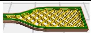 | 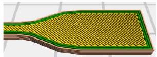 |
| Numerical result | 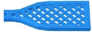 | 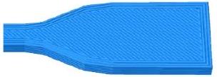 |
| Orientation | | |
| | ( $0^{\circ} / 90^{\circ}$ ) | ( $90^{\circ} / 0^{\circ}$ ) |
| Slicer result | 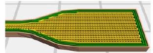 | 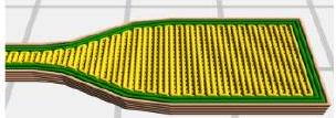 |
| Numerical result | 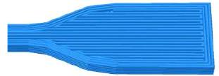 | 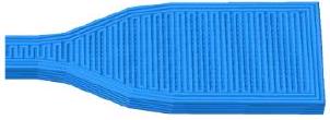 |
| External layer | | |
| | One | Three |
| Slicer result | 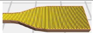 | 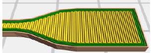 |
| Numerical result | 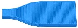 | 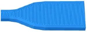 |
| Infill pattern | | |
| | Honeycomb (Hexagonal) | Triangular |
| Slicer result | 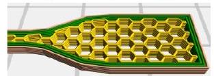 | 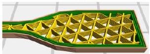 |
| Numerical result | 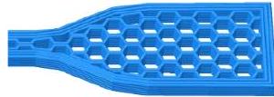 | 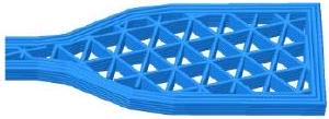 |
Figure 11: Comparison between Abaqus simulations and slicer-generated geometries.
The comparison of the 3D structures created in Abaqus (after going through G-code processing) with the true geometries of the original G-code produced through the slicing software validates the geometrical accuracy of this technique.
The superimposed 3D specimen representations shown in Fig. 11 prove that the resultant geometries produced in the slicer (at the bottom of the figure) for the various patterns of infill (honeycomb, grid, and linear) have precisely the same geometry as those obtained from Abaqus simulations. Each of these geometries has been created using identical wall layer compositions, densities, and orientations. In other words, the tool correctly replicates complex internal structures without any deviation or loss of detail. This establishes that the conversion between G-code and Abaqus is accurate, allowing for no detectable differences among the three sources and therefore providing confidence in the ability of the tool to maintain the integrity of a given design. Because of this high level of fidelity between printed items and simulated specimens, the mechanical properties of FDM parts can be reliably evaluated through simulation, making them suitable for critical applications.
Numerical model validation
Two separate sets of numerical tensile test simulations for ASTM D638 specimens were developed based on the uncorrected circular virtual section of similar shape as the nominal nozzle and an oval-rectangular virtual section which was calibrated through experimental means. No changes in virtual section size were accounted for the entire length of the filament, which is why all of the simulations were treated the same to keep them consistent. All simulations also took place at room temperature and the temperature effect due to an electrical build platform was negligible. The material properties of the ABS Monofilament remained constant throughout the simulation. This assumes that there would be no change in ABS material properties during the extrusion process. Fig. 12 is an example of a numerical tensile test set-up in Abaqus of an ASTM D638 specimen. One side of the model is anchored ("Encastred") while the other side is subjected to a specified amount of displacement according to the experimental data collected for the particular specimen. This model employs C3D4 linear tetrahedral elements measuring 0.55 mm based on convergence tests that were completed prior to conducting simulations.
Figure 12: Tensile test mesh setup for ASTM D638 specimens.
Fig. 13 compares stress-strain responses of ASTM D638 tensile specimens across three filament orientations (0^(@),45^(@),90^(@))\left(0^{\circ}, 45^{\circ}, 90^{\circ}\right). Each orientation subplot shows three experimental repetitions (green, teal, olive curves) and two simulation results:
"Numerical test (Corrected)" (blue circles) using the experimentally calibrated virtual section, and "Numerical test (nonCorrected)" (red triangles) using nominal circular cross-sections.
For the 0^(@)0^{\circ} orientation, the corrected numerical model demonstrates exceptional agreement with experimental results throughout the entire stress-strain curve. In the elastic region of the stress-strain relationship (when the strain is less than 0.005 ), both corrected and experimental data have very similar slopes and provide an accurate prediction of Young's modulus at approximately 2190 MPa . The corrected model remains very close in value leading up to the yield point (approximately 0.005 strain, 16 MPa stress) as well as in the plastic deformation region. The corrected simulation was able to predict the ultimate tensile strength (UTS) with great accuracy; the experimental UTS values fall between 41.4 to 41.5 MPa, while the corrected model yielded a UTS value of 41.4 MPa . The non-corrected model significantly underpredicts strength in the plastic region, with an approximate 15%15 \% difference from the maximum load. Similarly, for the 45^(@)45^{\circ} orientation, the corrected numerical model shows excellent correlation with experimental data regarding Young's Modulus and UTS predictions. Experimental UTS values fall between 38.0 to 38.5 MPa , while the corrected model yields results of approximately 38.5 MPa . The non-corrected model consistently underpredicts strength in the plastic region, with a deviation of approximately 5 to 8%8 \% from the maximum load. For the 90^(@)90^{\circ} raster orientation, the corrected and experimental data show close correlation again; the Young's modulus prediction of approximately 2190 MPa is within +-2\pm 2 to 3%3 \% of the stress measured during testing, thus confirming accurate stiffness modeling. The corrected simulation provides a good fit to the experimental stress drops and ductility in the plastic region, whereas the non-corrected model significantly under-predicts strength and does not reflect true failure mode. The experimental UTS ranged from 30.6 to 32.0 MPa in testing, whereas the corrected simulation achieved UTS results of between 30.8 to 32.5 MPa (less than 1%1 \% error), and the non-corrected model under-predicted by 10 to 15%15 \% ( 27.0 to 29.0 MPa ).
Figure 13: Comparative stress-strain curves of ASTM D638 specimens at (a) 0^(@)0^{\circ}, (b) 45^(@)45^{\circ}, and (c) 90^(@)90^{\circ} orientations: corrected vs. noncorrected numerical models and experimental results.
Across all tested raster orientations ( 0^(@),45^(@)0^{\circ}, 45^{\circ}, and 90^(@)90^{\circ} ), the corrected virtual section model demonstrates a consistently superior predictive capability compared to the non-corrected approach. For the 0^(@)0^{\circ} orientation, the corrected model achieves near-perfect replication of experimental stress-strain responses, including elastic modulus, yield point, ultimate tensile strength, and fracture strain, while the non-corrected model underestimates plastic performance by ∼15%\sim 15 \%. At 45^(@)45^{\circ}, the corrected model again captures both strength and ductility within experimental bounds, accurately reproducing gradual postUTS softening and matching failure strains, whereas the non-corrected approach introduces systematic underestimations.
For the 90^(@)90^{\circ} orientation, the corrected model successfully represents the brittle fracture governed by weak interlayer adhesion, predicting UTS and elongation with < 1-5%<1-5 \% error, while the non-corrected model overestimates ductility and underpredicts strength by 10-15%10-15 \%.
The simulation errors presented in Fig. 14 were rigorously calculated as the absolute and relative differences between the mean stress values from three repeated experimental tensile tests for each print orientation ( 0^(@),45^(@)0^{\circ}, 45^{\circ}, and 90^(@)90^{\circ} ) and the corresponding stress outputs from both the non-corrected and corrected virtual section finite element simulations at matching strain levels. Specifically, at each strain increment, the absolute error was computed as: (|Simulation Stress Experimental Mean Stress |) and the relative error by (|Simulation Stress - Experimental Mean Stress | / Experimental Mean Stress).
The comparative analysis of simulation errors across 0^(@),45^(@)0^{\circ}, 45^{\circ}, and 90^(@)90^{\circ} print orientations reveals a stark, quantifiable superiority of the corrected virtual section model over the non-corrected model not just in relative terms, but in absolute, engineering-critical values. In the 0^(@)0^{\circ} orientation, the non-corrected model begins with a catastrophic 100%100 \% relative error and stabilizes at an unacceptable 7-8%(~~2.5MPa7-8 \%(\approx 2.5 \mathrm{MPa} absolute error), systematically over-predicting stiffness due to incorrect moment of inertia. In contrast, the corrected model rapidly converges to near-perfect accuracy, finishing with a remarkable 0.1%0.1 \% relative error a 70-80x70-80 \mathrm{x} improvement. The 45^(@)45^{\circ} orientation, dominated by inter-raster shear, exposes even more dramatic failure: the non-corrected model's error explodes to 78%78 \% relative ( ~~14.5MPa\approx 14.5 \mathrm{MPa} ), dwarfing the material's actual strength ( 35-40MPa35-40 \mathrm{MPa} ), while the corrected model maintains a stable, engineering-acceptable 7%7 \% relative error (peak 1.3 MPa ), decreasing as deformation progresses. Most severely, in the 90^(@)90^{\circ} orientation the ultimate test of inter-layer adhesion the non-corrected model starts at an impossible 163%163 \% error and escalates to 92%(~~19MPa)92 \%(\approx 19 \mathrm{MPa}), predicting near-double the actual material strength, rendering it physically meaningless. Meanwhile, the corrected model plunges to a near-zero minimum of 0.03%0.03 \% relative error and remains under 10%10 \% throughout, accurately capturing delamination mechanics. Across all orientations, the non-corrected model consistently fails with errors ranging from 7%7 \% to 92%(2.5-19MPa)92 \%(2.5-19 \mathrm{MPa}), while the corrected model delivers precision within 0.03%0.03 \% to 7%( <= 1.3MPa)7 \%(\leq 1.3 \mathrm{MPa}), demonstrating not incremental but transformative accuracy. This proves the corrected model is not merely "better" it is the only version capable of reliable, predictive simulation for real-world additive manufacturing applications.
Across all orientations, the consistent pattern is clear: the non-corrected model fails quantitatively and physically, while the corrected model calibrated to real filament geometry delivers predictive accuracy validated against the statistical mean of experimental reality.
Figure 14: Comparative relative and absolute simulation errors vs. experimental mean ( n=3\mathrm{n}=3 ) across print orientations ( 0^(@),45^(@),90^(@)0^{\circ}, 45^{\circ}, 90^{\circ} ) noncorrected vs. corrected virtual section models.
Although a sample size of n=3\mathrm{n}=3 per orientation provides limited statistical power compared to conventional testing standards, this approach represents a balanced experimental design considering the resource-intensive nature of printing and testing FDM specimens with precisely controlled parameters. To address this limitation, we report 95%95 \% confidence intervals for all mean values and have focused our validation on consistent directional trends across orientations rather than absolute statistical significance. Our error analysis specifically compares simulation outputs to the experimental mean rather than individual specimens, acknowledging the inherent variability in FDM processes. Future work will expand the sample size and incorporate statistical design principles to better quantify process variability.
Conclusion
This study successfully developed and validated an experimentally calibrated methodology to significantly enhance the predictive accuracy of finite element simulations for Fused Deposition Modeling (FDM) components in Abaqus. The core innovation lies in replacing the conventional, idealized circular filament cross-section with a physically accurate "corrected virtual raster section," whose dimensions are predicted by a mathematical model derived from a systematic Box-Behnken Design of Experiments.
An Experimental analysis via SEM revealed that the true filament cross-section deviates significantly from the nominal circular shape, adopting an oval-rectangular profile due to extrusion-induced flattening and spreading. A
robust mathematical model was established to precisely quantify how critical printing parameters govern the final dimensions of this virtual section.
A custom Python-based interface was created to seamlessly parse G-code toolpaths and sweep the calibrated virtual section along the deposition trajectories. This automated workflow generates high-fidelity, mesh-ready Abaqus models that accurately represent the internal geometry and anisotropic nature of FDM-printed parts, as confirmed by perfect geometrical alignment with slicer-generated designs.
The tensile testing of ASTM D638 specimens demonstrated a transformative reduction in simulation error. The non-corrected model, using a nominal circular section, produced catastrophic and physically meaningless errors ranging from 7%7 \% to 92%92 \% ( 2.5-19MPa2.5-19 \mathrm{MPa} absolute). In stark contrast, the corrected model reduced these errors to engineering-grade precision, achieving a remarkable 0.03%0.03 \% to 7%7 \% relative error ( <= 1.3MPa\leq 1.3 \mathrm{MPa} absolute) across 0^(@),45^(@)0^{\circ}, 45^{\circ}, and 90^(@)90^{\circ} raster orientations.
The experimentally calibrated virtual raster section effectively captures the fundamental physics of filament deposition, enabling simulations that faithfully predict the mechanical performance and inherent anisotropy of FDM-printed structures. This work addresses a critical gap in the digital thread for additive manufacturing, offering a powerful tool for the design, optimization, and virtual qualification of 3D-printed components without the immediate need for extensive physical testing. While this study specifically demonstrated our approach using ABS material on a FlashForge Creator Pro printer with FlashPrint slicer, the fundamental methodology is broadly applicable to other FDM systems. The critical requirement for generalization is recalibration of the virtual raster section model for each material-printer combination through a reduced experimental design
[1] Bacciaglia, A., Falcetelli, F., Troiani, E., Di Sante, R., Liverani, A., Ceruti, A. (2023). Geometry reconstruction for additive manufacturing: From G-CODE to 3D CAD model, Mater Today Proc, 75, pp. 16-22.
DOI: https://doi.org/10.1016/J.MATPR.2022.09.496.
[2] Brenken, B., Barocio, E., Favaloro, A., Kunc, V., Pipes, R.B. (2019). Development and validation of extrusion deposition additive manufacturing process simulations, Addit Manuf, 25, pp. 218-226.
DOI: https://doi.org/10.1016/j.addma.2018.10.041.
[3] Cattenone, A., Morganti, S., Alaimo, G., Auricchio, F. (2018). Finite Element Analysis of Additive Manufacturing Based on Fused Deposition Modeling: Distortions Prediction and Comparison With Experimental Data, J Manuf Sci Eng, 141(1). DOI: https://doi.org/10.1115/1.4041626.
[4] Faria, C., Fonseca, J., Bicho, E. (2020). FIBR3DEmul-an open-access simulation solution for 3D printing processes of FDM machines with 3+3+ actuated axes, The International Journal of Advanced Manufacturing Technology, 106(7), pp. 3609-3623. DOI: https://doi.org/10.1007/s00170-019-04713-y.
[5] Gamdha, D., Saurabh, K., Ganapathysubramanian, B., Krishnamurthy, A. (2025). High-resolution thermal simulation framework for extrusion-based additive manufacturing of complex geometries, Finite Elements in Analysis and Design, 251, p. 104410. DOI: https://doi.org/10.1016/J.FINEL.2025.104410.
[6] Hachimi, T., Ait Hmazi, F., Majid, F. (2025). Damage of additively manufactured polymer materials: experimental and probabilistic analysis, Fracture and Structural Integrity, 19(73), pp. 236-255.
DOI: https://doi.org/10.3221/IGF-ESIS.73.16.
[7] Hachimi, T., Hmazi, F.A., Arhouni, F.E., Rejdali, H., Riyad, Y., Majid, F. (2025). Advancing FDM 3D Printing Simulations: From G-Code Conversion to Precision Modelling in Abaqus, Journal of Manufacturing and Materials Processing 2025, Vol. 9, Page 338, 9(10), p. 338. DOI: https://doi.org/10.3390/JMMP9100338.
[8] Hachimi, T., Majid, F., Zekriti, N., Rhanim, R., Rhanim, H. (2024). Improvement of 3D printing polymer simulations considering converting G-code to Abaqus, The International Journal of Advanced Manufacturing Technology, 131(9), pp. 5193-5208. DOI: https://doi.org/10.1007/s00170-024-13300-9.
[9] Hachimi, T., Zekriti, N., Rhanim, R., Rhanim, H., Majid, F. (2025). Modeling and Simulation of the Influence of 3D Printing Parameters on Crack Propagation: Filament Orientation., In: Boutahir, M., El Mehdi, E. eds., Advanced Materials for Sustainable Energy and Engineering: Volume 1: Novel Nanomaterials for Sustainable Energy, Cham, Springer Nature Switzerland, pp. 231-245.
[10] Kechagias, J.D. (2024). 3D printing parametric optimization using the power of Taguchi design: an expository paradigm, Materials and Manufacturing Processes, 39(6), pp. 797-803. DOI: https://doi.org/10.1080/10426914.2023.2290258.
[11]Mishra, V., Negi, S., Kar, S. (2023). FDM-based additive manufacturing of recycled thermoplastics and associated composites, J Mater Cycles Waste Manag, 25(2), pp. 758-784.
[12] Molazadeh, S., Diba, F., Hosseini, A. (2023). Anisotropic modeling of material behavior for additively manufactured parts made by material extrusion, International Journal of Advanced Manufacturing Technology, 129(7-8), pp. 34533473. DOI: https://doi.org/10.1007/S00170-023-12508-5/METRICS.
[13] Montalti, A., Ferretti, P., Santi, G.M. (2024). From CAD to G-code: Strategies to minimizing errors in 3D printing process, CIRP J Manuf Sci Technol, 55, pp. 62-70. DOI: https://doi.org/10.1016/J.CIRPJ.2024.09.005.
[14] Moradi, M., Hashemi, R., Kasaeian-Naeini, M. (2023). Experimental investigation of parameters in fused filament fabrication 3D printing process of ABS plus using response surface methodology, The International Journal of Advanced Manufacturing Technology 2023, pp. 1-18. DOI: https://doi.org/10.1007/S00170-023-11468-0.
[15] Naboulsi, N., Hachimi, T., Majid, F., Rhanim, R., Zekriti, N., Rhanim, H. (2021). Modeling and control of 3D filament extruder., Procedia Structural Integrity, 33.
[16] Naboulsi, N., Majid, F., Hachimi, T., Dadoun, S., Barhoumi, N., Khlifi, K. (2025). Predicting the strength of 3D-printed conductive composite under tensile load: A probabilistic modeling and experimental study, Fracture and Structural Integrity, 19(72), pp. 247-262. DOI: https://doi.org/10.3221/IGF-ESIS.72.18.
[17] Pal, A.K., Mohanty, A.K., Misra, M. (2021). Additive manufacturing technology of polymeric materials for customized products: recent developments and future prospective, RSC Adv, 11(58), pp. 36398-36438.
DOI: https://doi.org/10.1039/D1RA04060J.
[18] Pereira, T., Kennedy, J. V., Potgieter, J. (2019). A comparison of traditional manufacturing vs additive manufacturing, the best method for the job, Procedia Manuf, 30, pp. 11-18. DOI: https://doi.org/10.1016/J.PROMFG.2019.02.003.
[19] Picard, M., Mohanty, A.K., Misra, M. (2020). Recent advances in additive manufacturing of engineering thermoplastics: Challenges and opportunities, RSC Adv, 10(59), pp. 36058-36089. DOI: https://doi.org/10.1039/D0RA04857G.
[20] R, R.M., R, V., S, R. (2021). Experimental analysis on density, micro-hardness, surface roughness and processing time of Acrylonitrile Butadiene Styrene (ABS) through Fused Deposition Modeling (FDM) using Box Behnken Design (BBD), Mater Today Commun, 27, p. 102353. DOI: 10.1016/J.MTCOMM.2021.102353.
[21]Samykano, M., Selvamani, S.K., Kadirgama, K., Ngui, W.K., Kanagaraj, G., Sudhakar, K. (2019). Mechanical property of FDM printed ABS: influence of printing parameters, The International Journal of Advanced Manufacturing Technology, 102, pp. 2779-2796.
[22] Sola, A., Trinchi, A. (2022). Fused Deposition Modeling of Composite Materials, Fused Deposition Modeling of Composite Materials, pp. 1-448. DOI: https://doi.org/10.1016/C2021-0-00489-2.
[23] Taoufik, H., Fatima, M., Hassan, R. (2023). Modeling of the fracture behavior of the 3D Printed polymers using XFEM, Procedia Structural Integrity, 47, pp. 711-722. DOI: https://doi.org/10.1016/j.prostr.2023.07.048.
[24] Timofeeva, O.S., Andreev, Y.S., Yablochnikov, E.I. (2019). Simulation of injection molding process and 3D-printing of forming parts for small-batch production., 2019 IEEE 17th International Conference on Industrial Informatics (INDIN), 1, pp. 1631-1637.
[25] Vanaei, H.R., Khelladi, S., Tcharkhtchi, A. (2024). 3D printing as a multidisciplinary field, Industrial Strategies and Solutions for 3D Printing: Applications and Optimization, pp. 1-24.
DOI: https://doi.org/10.1002/9781394150335.CH1;CTYPE:STRING:BOOK.
[26] Yu, W., Shi, J., Sun, L., Lei, W. (2022). Effects of Printing Parameters on Properties of FDM 3D Printed Residue of Astragalus/Polylactic Acid Biomass Composites, Molecules, 27(21), p. 7373.
DOI: https://doi.org/10.3390/MOLECULES27217373.
[27] Zhang, Y., Huang, X. (2020). Simulation and Research of Aerospace Material Milling Based On ABAQUS, J Phys Conf Ser, 1653(1), p. 012070. DOI: https://doi.org/10.1088/1742-6596/1653/1/012070.
[28] Zouaoui, M., Gardan, J., Lafon, P., Makke, A., Labergere, C., Recho, N. (2021). A Finite Element Method to Predict the Mechanical Behavior of a Pre-Structured Material Manufactured by Fused Filament Fabrication in 3D Printing, Applied Sciences 2021, 11, pp. 5075. DOI: https://doi.org/10.3390/APP11115075.
[29] Zouaoui, M., Labergere, C., Gardan, J., Makke, A., Recho, N., Alexandre, Q., Lafon, P. (2019). Numerical prediction of 3d printed specimens based on a strengthening method of fracture toughness, Procedia CIRP, 81, pp. 40-44.




















